stan overview
Stan is a platform used for Bayesian modelling. Unlike JAGS and BUGS the underlying MCMC algorithm is Hamiltonian - meaning it uses gradients rather than steps. Stan uses a variant of a No-U-Turn Sampler (NUTS) to explore the target parameter space and return the model output.
In practice, this means:
- Better at exploring the model space
- More likely to find issues with the model parameterisation
- Quicker than JAGS/BUGS with more complex models
- LOADS of diagnostics
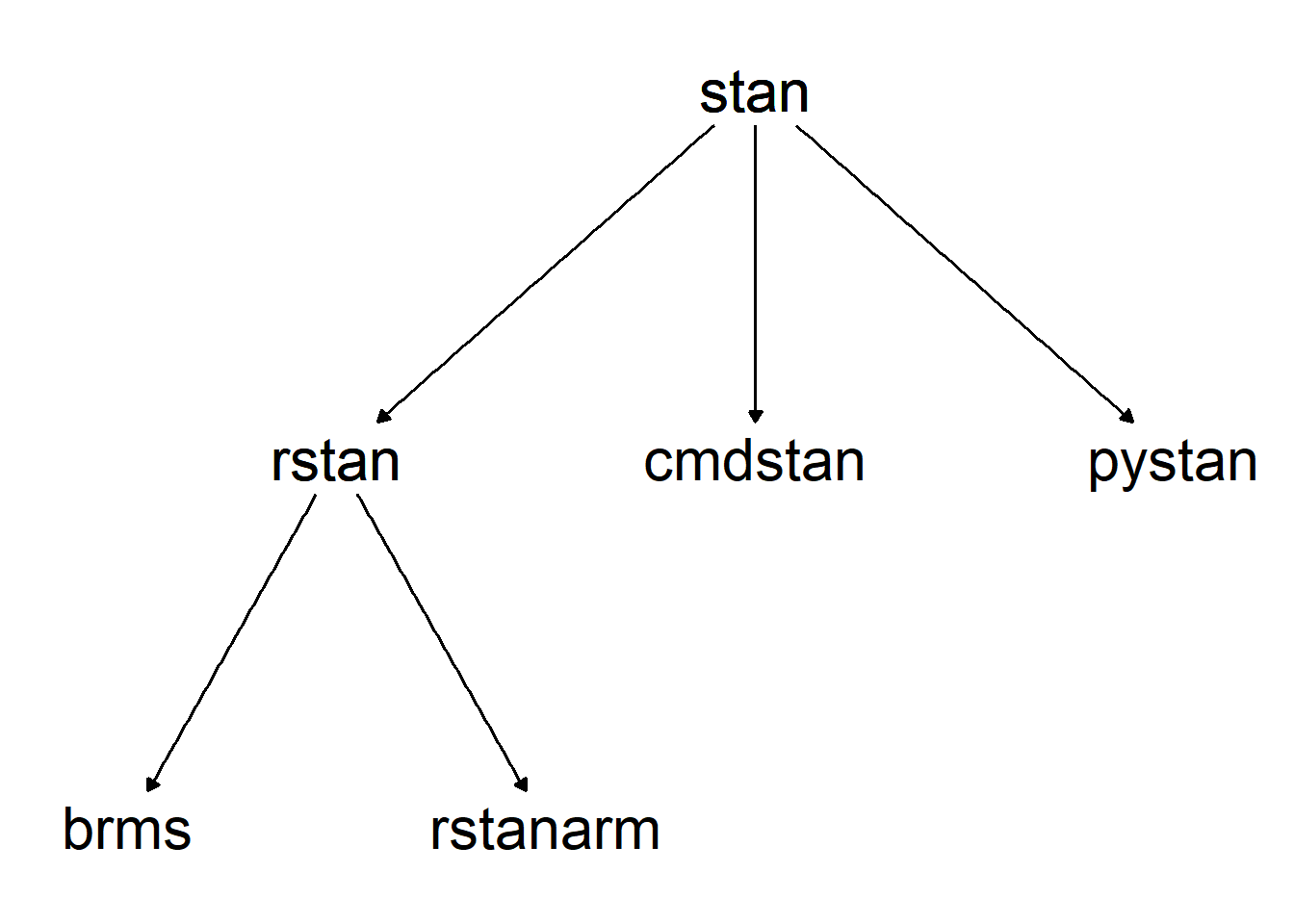
Stan can be interfaced to from various software, the most commonly used and well supported is R but there are also options to interface from python or the command line. Within R there is the rstan package which does the direct interfacing with stan (along with StanHeaders), but there are also many helper packages for fitting stan models including rstanarm and brms.
There are also several other packages in R that work with stan models, such as bayesplot, loo, shinystan etc.
Both rstanarm and brms use formula notation in the style of lme4 in order to specify stan models. The main difference in between the two packages is that rstanarm has all of their models pre-specified and compiled into stan code while brms writes and compiles a new stan model each time. This means rstanarm can be a lot quicker than brms, but brms supports a wider range of model types. I use brms exclusively as I am a creature of habit and learnt it first, so that is what I will present here.
Installation
A guide to installing rstan can be found online here, it is now much easier than it used to be - just install off CRAN as standard. It will take a few minutes, and afterwards you need to check whether your C++ toolchain is correctly set up using pkgbuild. Their github page also gives an optional step to configure the toolchain.
install.packages("rstan")

# check toolchain
pkgbuild::has_build_tools(debug = TRUE)

# Optional - configure toolchain
dotR <- file.path(Sys.getenv("HOME"), ".R")
if (!file.exists(dotR)) dir.create(dotR)
M <- file.path(dotR, ifelse(.Platform$OS.type == "windows", "Makevars.win", "Makevars"))
if (!file.exists(M)) file.create(M)
cat("\nCXX14FLAGS=-O3 -march=native -mtune=native",
    if( grepl("^darwin", R.version$os)) "CXX14FLAGS += -arch x86_64 -ftemplate-depth-256" else
    if (.Platform$OS.type == "windows") "CXX11FLAGS=-O3 -march=corei7 -mtune=corei7" else
    "CXX14FLAGS += -fPIC",
    file = M, sep = "\n", append = TRUE)
Other packages that rely on rstan can be installed from CRAN/github as usual, I won’t go into the details here.
library(brms)
library(dplyr)
library(ggplot2)
theme_set(theme_classic())
Simple model example
I’m going to start by running a very simple mixed model here in order to demonstrate how easy fitting a model with brms can be. All the data here is from the agridat package, which is a package that holds several agricultural related datasets.
library(agridat)
dat <- ilri.sheep
ggplot(dat, aes(x = gen, y = weanwt)) +
  geom_boxplot()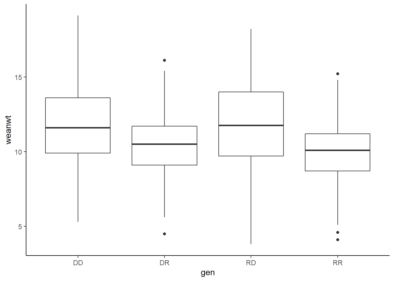
The brms model for this (with default priors, i.e. this is not a recommended workflow!):
mod1 <- brm(weanwt ~ gen - 1 + (1|ewe) + (1|ram), data = ilri.sheep, cores = 4)summary(mod1)## Family: gaussian
## Links: mu = identity; sigma = identity
## Formula: weanwt ~ gen - 1 + (1 | ewe) + (1 | ram)
## Data: ilri.sheep (Number of observations: 700)
## Samples: 4 chains, each with iter = 2000; warmup = 1000; thin = 1;
## total post-warmup samples = 4000
##
## Group-Level Effects:
## ~ewe (Number of levels: 358)
## Estimate Est.Error l-95% CI u-95% CI Rhat Bulk_ESS Tail_ESS
## sd(Intercept) 1.16 0.18 0.77 1.49 1.01 585 669
##
## ~ram (Number of levels: 74)
## Estimate Est.Error l-95% CI u-95% CI Rhat Bulk_ESS Tail_ESS
## sd(Intercept) 0.78 0.17 0.45 1.12 1.00 1080 1696
##
## Population-Level Effects:
## Estimate Est.Error l-95% CI u-95% CI Rhat Bulk_ESS Tail_ESS
## genDD 11.62 0.23 11.15 12.07 1.00 2585 3083
## genDR 10.61 0.31 10.01 11.23 1.00 3002 2905
## genRD 11.70 0.24 11.24 12.19 1.00 2213 2992
## genRR 9.82 0.26 9.29 10.34 1.00 2249 2310
##
## Family Specific Parameters:
## Estimate Est.Error l-95% CI u-95% CI Rhat Bulk_ESS Tail_ESS
## sigma 2.29 0.10 2.12 2.49 1.00 746 1086
##
## Samples were drawn using sampling(NUTS). For each parameter, Bulk_ESS
## and Tail_ESS are effective sample size measures, and Rhat is the potential
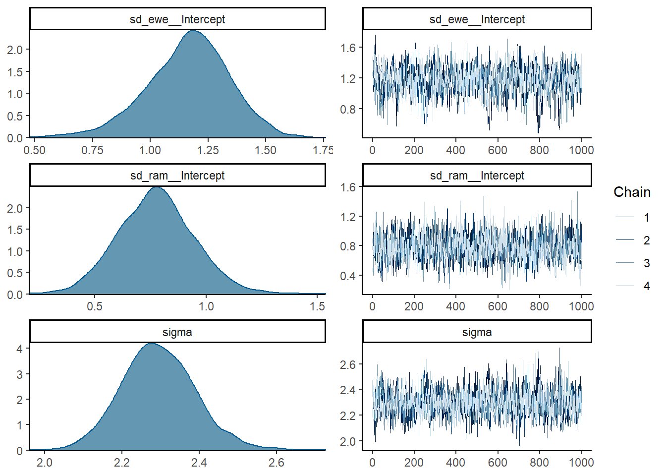
## scale reduction factor on split chains (at convergence, Rhat = 1).plot(mod1, ask = FALSE, N = 4)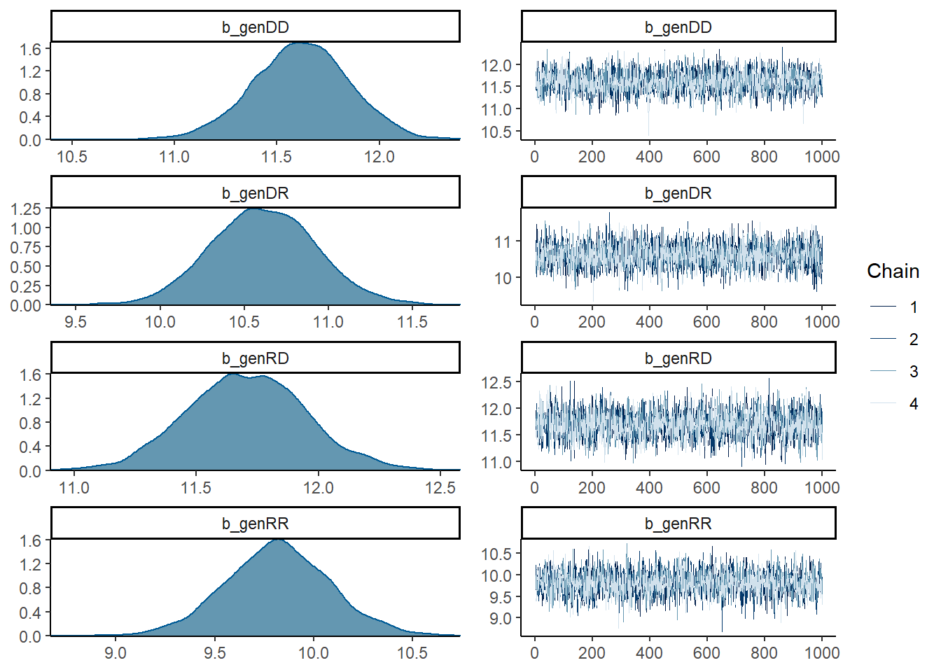
Example suggested workflow
When using these methods it is suggested that you think more about the prior assumptions that you are putting into the model. Several people within the stan community are now advocating a model building approach that follows several steps. I’m going to give a quick outline of the kind of steps that I follow when building models.
First, prior predictive checks. Here we take the model structure and priors we are suggesting and evaluate the data structure that is implied by these priors.
Binomial data - Phytophtera disease occurrence in a pepper field.
dat <- gumpertz.pepper %>%
  mutate(disease = recode(disease, "Y" = 1, "N" = 0))
ggplot(dat, aes(x = leaf, y = disease, colour = water)) + geom_jitter()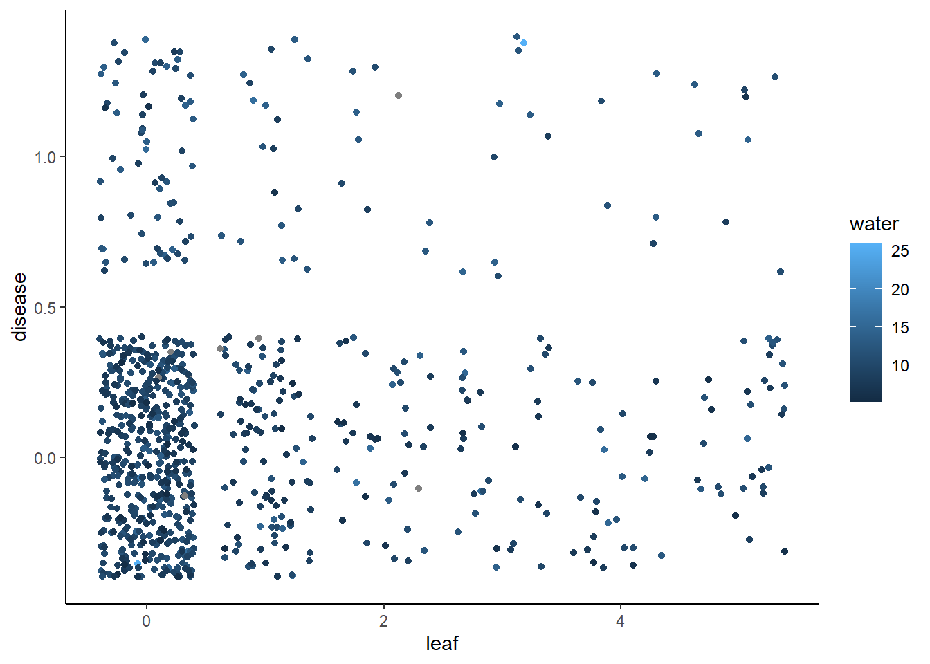
First, define the model and find out what priors are automatically given by brms.
get_prior(y ~ trt - 1 + (1|block), data = beall.webworms,
          family = poisson)
## prior class coef group resp dpar nlpar bound
## 1 b
## 2 b trtT1
## 3 b trtT2
## 4 b trtT3
## 5 b trtT4
## 6 student_t(3, 0, 2.5) sd
## 7 sd block
## 8 sd Intercept blockSo we can see that the default is to have a student T prior on the intercept and random effect. Let’s put a wide prior on b
pr <- prior(normal(0,10), class = "b")Now check by sampling the prior what kind of data this suggests:
mod_pr <- brm(y ~ trt - 1 + (1|block), data = beall.webworms,
              family = poisson, prior = pr,
              cores = 4, sample_prior = "only")
There is handy function within stan that allows you to see what the data suggested by the model looks like - pp_check. I will discuss this more later when we come to posterior checks but the default plots the density of the data and the model predicted data. You can also use plot(conditional_effects(
pp_check(mod_pr)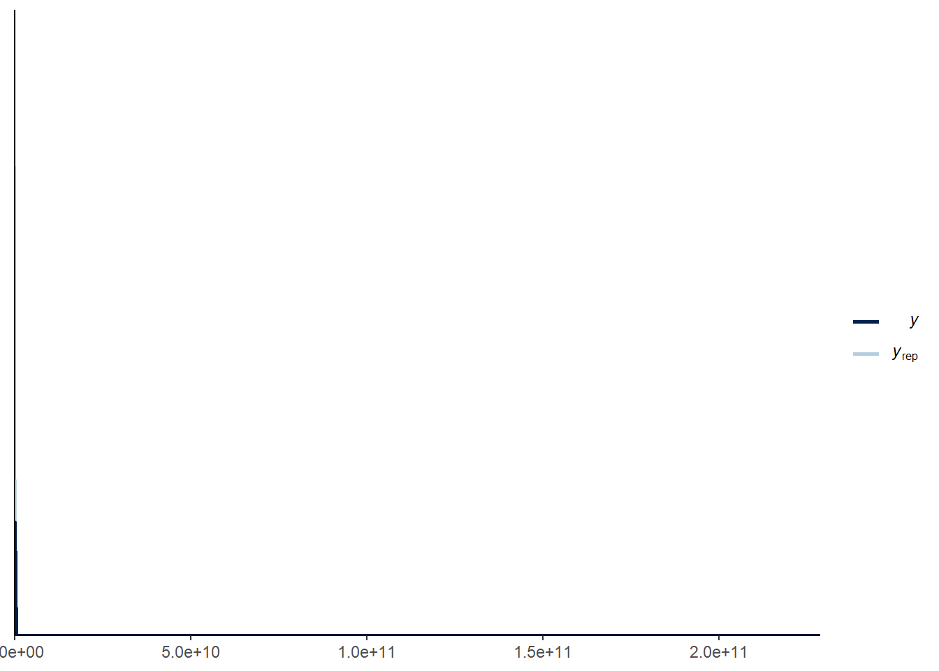
plot(conditional_effects(mod_pr))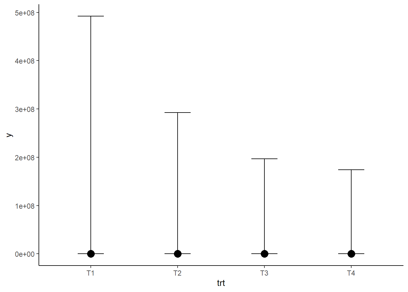
These plots show that our prior suggests that having counts of millions/billions is a possible outcome, which both seems unreasonable and could lead to issues with model convergence as the model fitting process has to explore these unlikely regions of model space. We can try this with tighter priors and see if it makes the model more sensible.
pr <- prior(normal(0,.5), class = "b") +
  prior(student_t(3,0,1), class = "sd") +
  prior(student_t(3,0,1), class = "Intercept")
Now check by sampling the prior what kind of data this suggests
mod_pr <- update(mod_pr, prior = pr, cores = 4, sample_prior = "only")pp_check(mod_pr)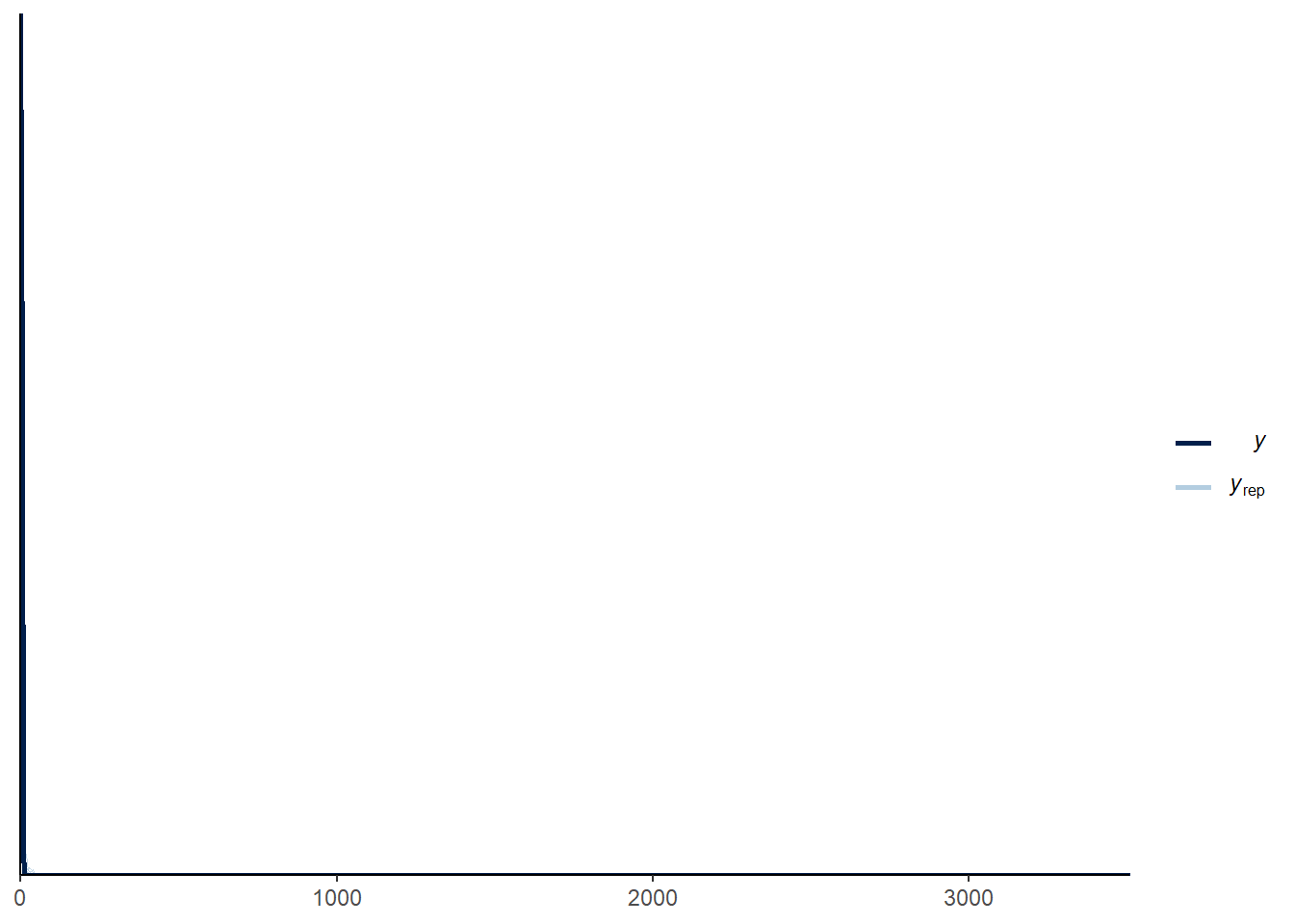
This prior seems really tight but actually allows for pretty high counts. Now we can run the model with data:
mod_p <- update(mod_pr, sample_prior = "no", cores = 4)Model checks!
Statistics are printed by summary
summary(mod_p)## Family: poisson
## Links: mu = log
## Formula: y ~ trt - 1 + (1 | block)
## Data: beall.webworms (Number of observations: 1300)
## Samples: 4 chains, each with iter = 2000; warmup = 1000; thin = 1;
## total post-warmup samples = 4000
##
## Group-Level Effects:
## ~block (Number of levels: 13)
## Estimate Est.Error l-95% CI u-95% CI Rhat Bulk_ESS Tail_ESS
## sd(Intercept) 0.39 0.10 0.24 0.63 1.00 686 1051
##
## Population-Level Effects:
## Estimate Est.Error l-95% CI u-95% CI Rhat Bulk_ESS Tail_ESS
## trtT1 0.34 0.11 0.14 0.56 1.00 767 966
## trtT2 -0.67 0.12 -0.90 -0.41 1.00 917 1081
## trtT3 -0.15 0.11 -0.37 0.09 1.00 829 1084
## trtT4 -0.86 0.13 -1.10 -0.59 1.00 946 1155
##
## Samples were drawn using sampling(NUTS). For each parameter, Bulk_ESS
## and Tail_ESS are effective sample size measures, and Rhat is the potential
## scale reduction factor on split chains (at convergence, Rhat = 1).Plot the variables to see the traceplots
plot(mod_p)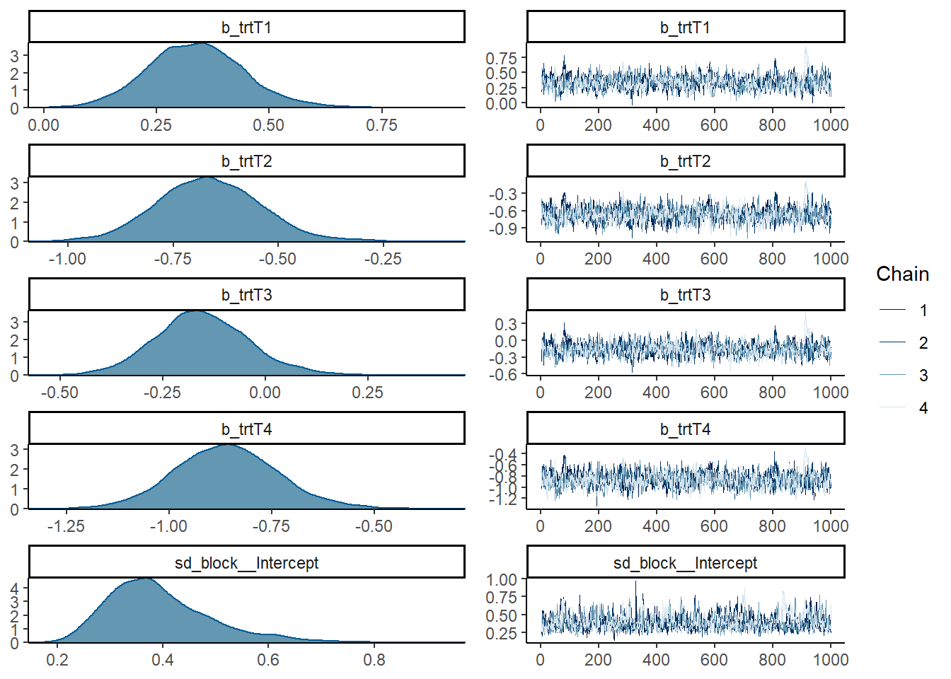
Alternatively, plot the rank overlay for the chains
mcmc_plot(mod_p, type = "rank_overlay")
Now we can look at how well the model predicted the data using posterior predictive checks:
pp_check(mod_p)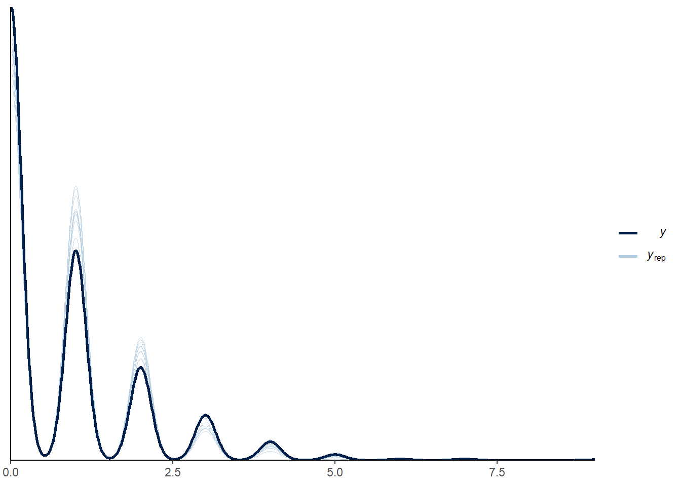
There are other types of posterior predictive checks supported by pp_check, described further in the documentation.
To examine what the model estimates the effect of treatment to be upon worm count we can plot the predicted response for the different predictors.
fixef(mod_p)## Estimate Est.Error Q2.5 Q97.5
## trtT1 0.3383876 0.1086578 0.1363769 0.56392432
## trtT2 -0.6658319 0.1235601 -0.8990215 -0.41407681
## trtT3 -0.1534075 0.1145232 -0.3690580 0.08595225
## trtT4 -0.8588937 0.1268969 -1.1013487 -0.59478242plot(conditional_effects(mod_p))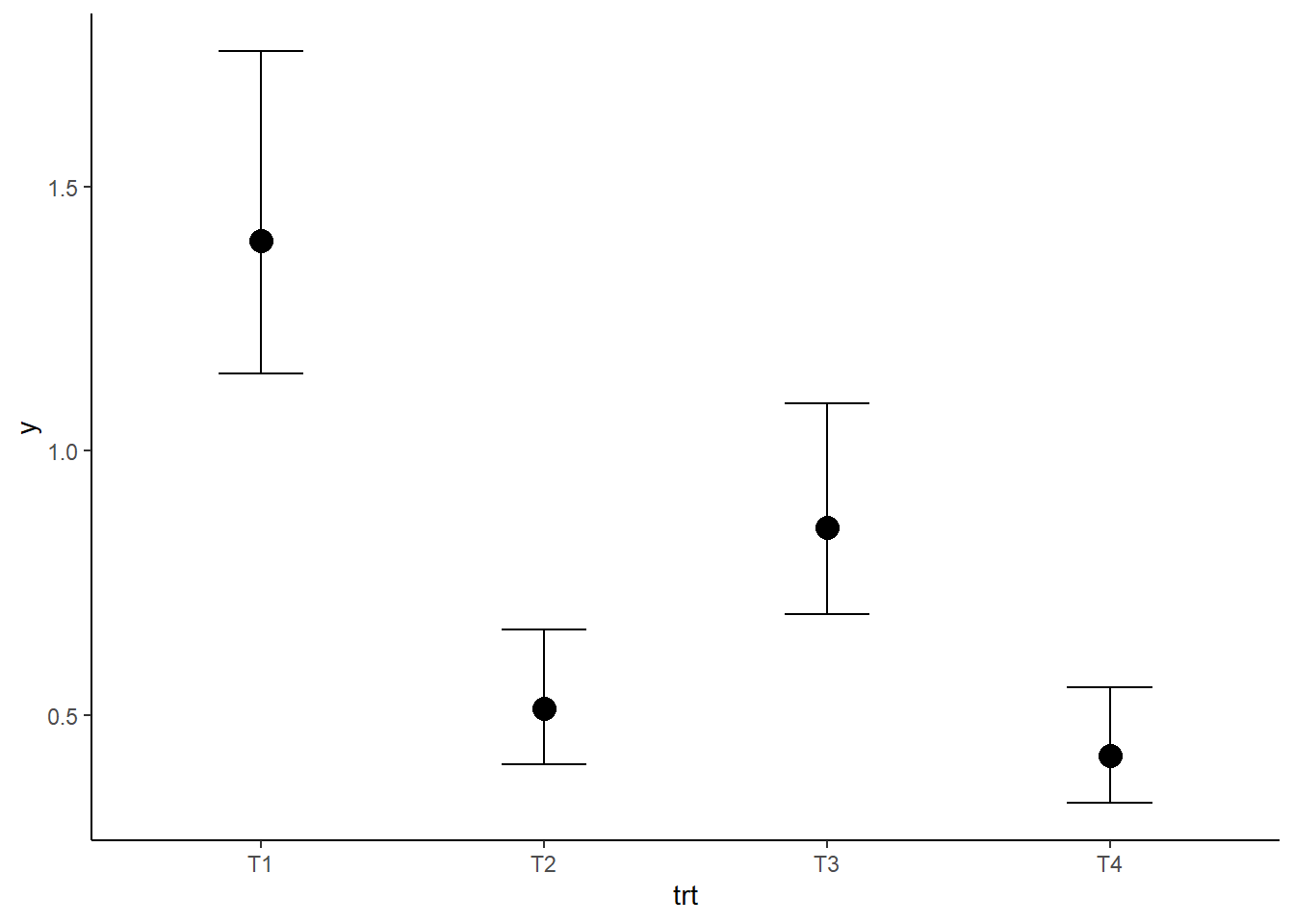
Errors
Stan returns many more potential errors and warnings than other MCMC software, in part because the fine-tuning of the NUTS algorithm offers more opportunities to pick up on issues with the exploration of model space. A full description of the different warnings is at https://mc-stan.org/misc/warnings.html but here’s a quick summary of the ones I’ve commonly run into:
- divergent transitions - the warning message will recommend increasing adapt_delta which may work, if not then the model structure needs to change
- maximum treedepth exceeded - the warning message will recommend increasing max_treedepth (this is an efficiency concern, not a validity concern)
- Rhat - will return a warning if above 1.05. Note that stan now uses a more robust rhat so this will pick up on issues where the old version may not have.
- Effective sample size warnings for the bulk and tail of the distribution, will suggest running for more iterations but I’ve mostly run across these when chains haven’t fully converged so fix that first
More complicated models
The above are quite simple examples, but brms can support many other types of model including those with missing data, censoring, multiple responses or non-linear models.
Multivariate models
Modelling multiple response variables within brms can be done in one of two ways, if you have both response variables being predicted by the same predictors and having the same family you can use mvbind() to combine the two. Otherwise, you have to specify each formula within a bf() function then combine them together in the brm call. Fitting multiple models together allows you to model correlation between response variables and use information criteria or cross-validation upon the entire model.
dat <- australia.soybean %>%
  mutate(YR = as.factor(year)) %>%
  mutate_if(is.numeric, scale) %>%
  na.omit()

pr <- c(prior(normal(0,1), class = "b", resp = "protein"),
        prior(normal(0,1), class = "b", resp = "oil"))

mod_mv <- brm(mvbind(protein,oil) ~ year*loc,
              data = dat, prior = pr, cores = 4)
summary(mod_mv)
## Family: MV(gaussian, gaussian)
## Links: mu = identity; sigma = identity
## mu = identity; sigma = identity
## Formula: protein ~ year * loc
## oil ~ year * loc
## Data: dat (Number of observations: 464)
## Samples: 4 chains, each with iter = 2000; warmup = 1000; thin = 1;
## total post-warmup samples = 4000
##
## Population-Level Effects:
## Estimate Est.Error l-95% CI u-95% CI Rhat Bulk_ESS
## protein_Intercept 0.20 0.07 0.05 0.34 1.00 2120
## oil_Intercept -0.25 0.08 -0.40 -0.09 1.00 2195
## protein_year 0.29 0.07 0.14 0.44 1.00 1675
## protein_locLawes -0.38 0.11 -0.59 -0.18 1.00 2314
## protein_locNambour -0.66 0.10 -0.87 -0.46 1.00 2481
## protein_locRedlandBay 0.26 0.11 0.05 0.47 1.00 2630
## protein_year:locLawes -0.21 0.11 -0.42 -0.01 1.00 1867
## protein_year:locNambour 0.44 0.11 0.23 0.65 1.00 2240
## protein_year:locRedlandBay 0.07 0.10 -0.14 0.28 1.00 2026
## oil_year -0.12 0.08 -0.28 0.03 1.00 1625
## oil_locLawes 0.34 0.11 0.11 0.56 1.00 2469
## oil_locNambour 0.78 0.11 0.56 1.01 1.00 2556
## oil_locRedlandBay -0.13 0.12 -0.36 0.09 1.00 2763
## oil_year:locLawes -0.06 0.12 -0.29 0.15 1.00 1826
## oil_year:locNambour -0.37 0.11 -0.61 -0.15 1.00 2228
## oil_year:locRedlandBay 0.07 0.11 -0.16 0.30 1.00 2042
## Tail_ESS
## protein_Intercept 2620
## oil_Intercept 2682
## protein_year 2444
## protein_locLawes 3076
## protein_locNambour 3224
## protein_locRedlandBay 2995
## protein_year:locLawes 2824
## protein_year:locNambour 2974
## protein_year:locRedlandBay 2215
## oil_year 2581
## oil_locLawes 3106
## oil_locNambour 3096
## oil_locRedlandBay 3260
## oil_year:locLawes 2357
## oil_year:locNambour 2701
## oil_year:locRedlandBay 2340
##
## Family Specific Parameters:
## Estimate Est.Error l-95% CI u-95% CI Rhat Bulk_ESS Tail_ESS
## sigma_protein 0.83 0.03 0.78 0.89 1.00 2849 3088
## sigma_oil 0.90 0.03 0.84 0.96 1.00 3165 2608
##
## Residual Correlations:
## Estimate Est.Error l-95% CI u-95% CI Rhat Bulk_ESS Tail_ESS
## rescor(protein,oil) -0.71 0.02 -0.75 -0.66 1.00 3072 2901
##
## Samples were drawn using sampling(NUTS). For each parameter, Bulk_ESS
## and Tail_ESS are effective sample size measures, and Rhat is the potential
## scale reduction factor on split chains (at convergence, Rhat = 1).plot(conditional_effects(mod_mv, effects = "year:loc", resp = "protein"))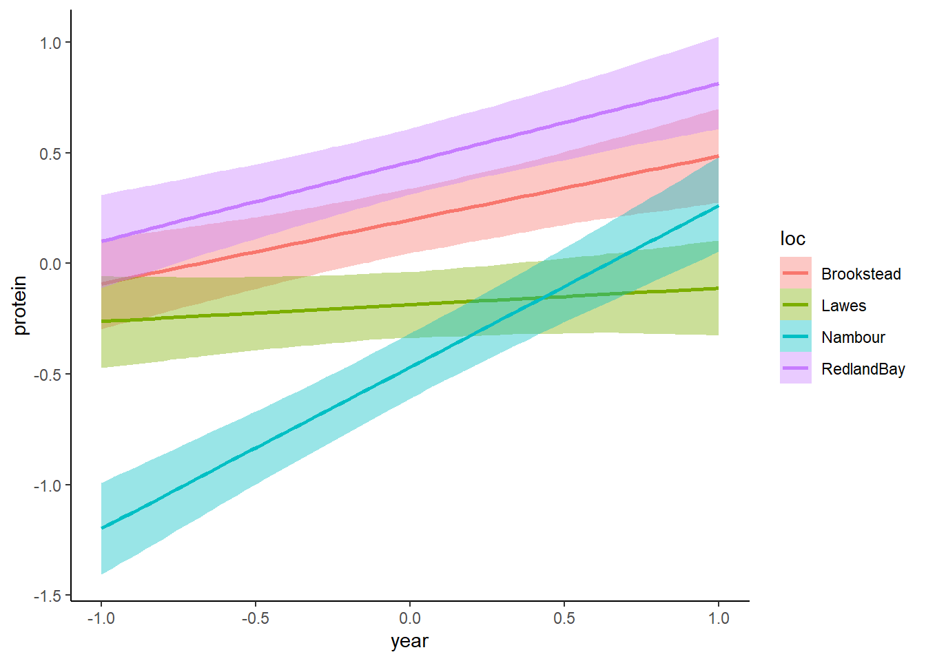
plot(conditional_effects(mod_mv, effects = "year:loc", resp = "oil"))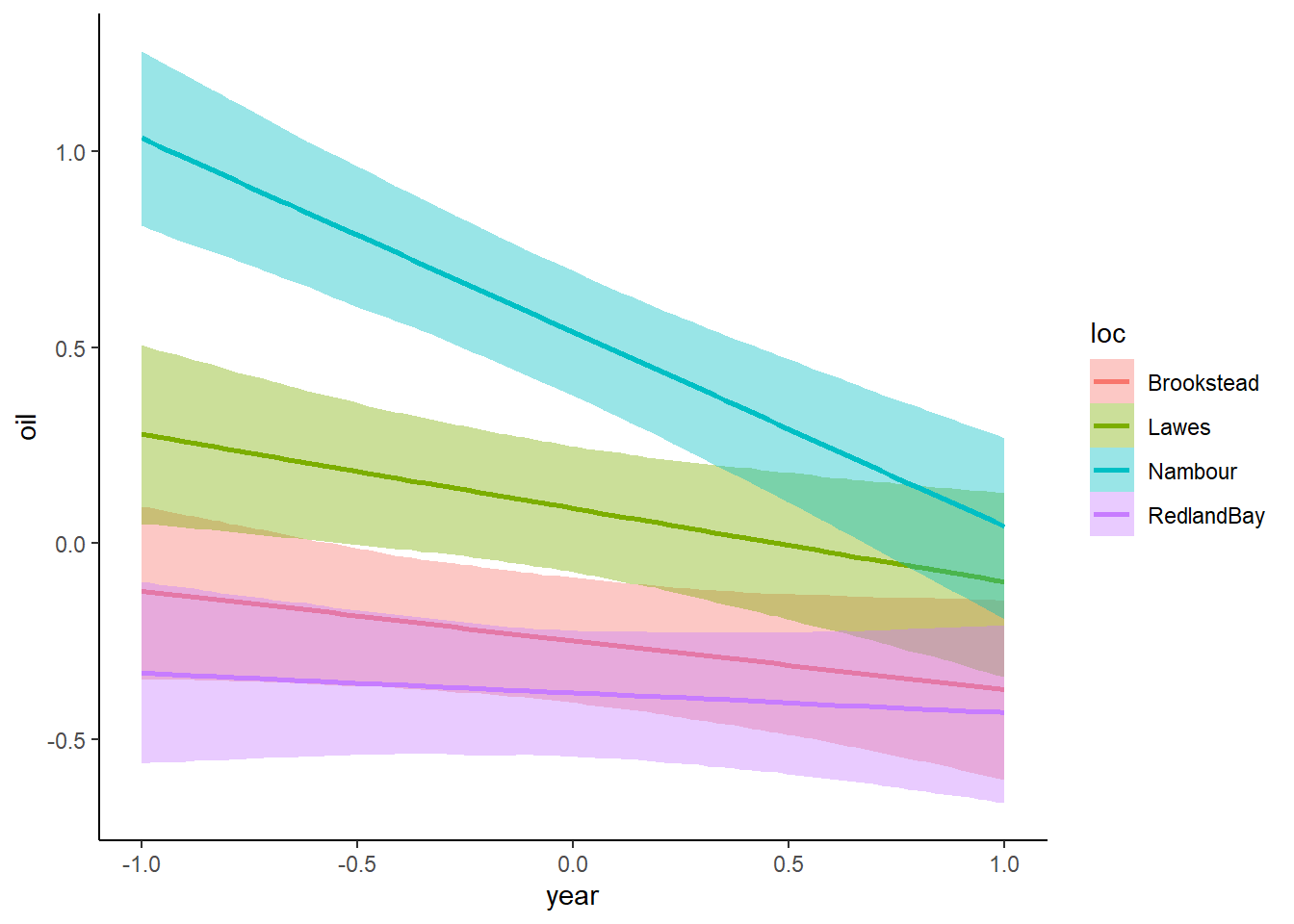
mod_mv <- add_criterion(mod_mv, "loo")
print(mod_mv$criteria$loo)
##
## Computed from 4000 by 464 log-likelihood matrix
##
## Estimate SE
## elpd_loo -1029.2 20.0
## p_loo 18.1 0.9
## looic 2058.4 40.0
## ------
## Monte Carlo SE of elpd_loo is 0.1.
##
## All Pareto k estimates are good (k < 0.5).
## See help('pareto-k-diagnostic') for details.Alternatively, if the two response variables have differing
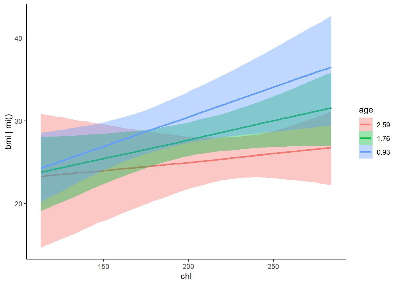
Missing data
Missing data can be imputed using the mi() notation, you have to specify which predictors you want the model to use in imputing the missing data. This example is lifted directly from the missing data vignette in brms.
data("nhanes", package = "mice")
bform <- bf(bmi | mi() ~ age * mi(chl)) +
  bf(chl | mi() ~ age) + set_rescor(FALSE)
fit <- brm(bform, data = nhanes, cores = 4)
summary(fit)
## Family: MV(gaussian, gaussian)
## Links: mu = identity; sigma = identity
## mu = identity; sigma = identity
## Formula: bmi | mi() ~ age * mi(chl)
## chl | mi() ~ age
## Data: nhanes (Number of observations: 25)
## Samples: 4 chains, each with iter = 2000; warmup = 1000; thin = 1;
## total post-warmup samples = 4000
##
## Population-Level Effects:
## Estimate Est.Error l-95% CI u-95% CI Rhat Bulk_ESS Tail_ESS
## bmi_Intercept 13.84 8.43 -3.58 30.32 1.00 1589 2120
## chl_Intercept 142.25 25.37 92.23 192.77 1.00 2972 2619
## bmi_age 2.69 5.32 -7.63 13.42 1.00 1252 1926
## chl_age 28.32 13.35 0.89 54.35 1.00 2907 2772
## bmi_michl 0.10 0.04 0.01 0.18 1.00 1728 1901
## bmi_michl:age -0.03 0.02 -0.08 0.02 1.00 1339 1991
##
## Family Specific Parameters:
## Estimate Est.Error l-95% CI u-95% CI Rhat Bulk_ESS Tail_ESS
## sigma_bmi 3.35 0.75 2.23 5.12 1.00 1509 2425
## sigma_chl 40.07 7.41 28.50 57.68 1.00 2081 2582
##
## Samples were drawn using sampling(NUTS). For each parameter, Bulk_ESS
## and Tail_ESS are effective sample size measures, and Rhat is the potential
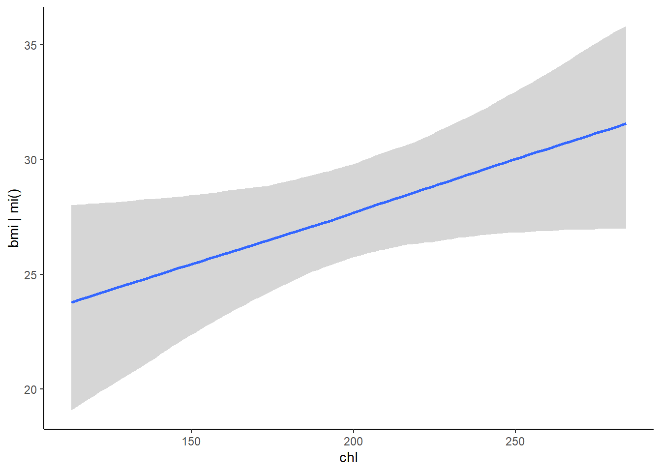
## scale reduction factor on split chains (at convergence, Rhat = 1).plot(conditional_effects(fit, resp = "bmi"), ask = FALSE)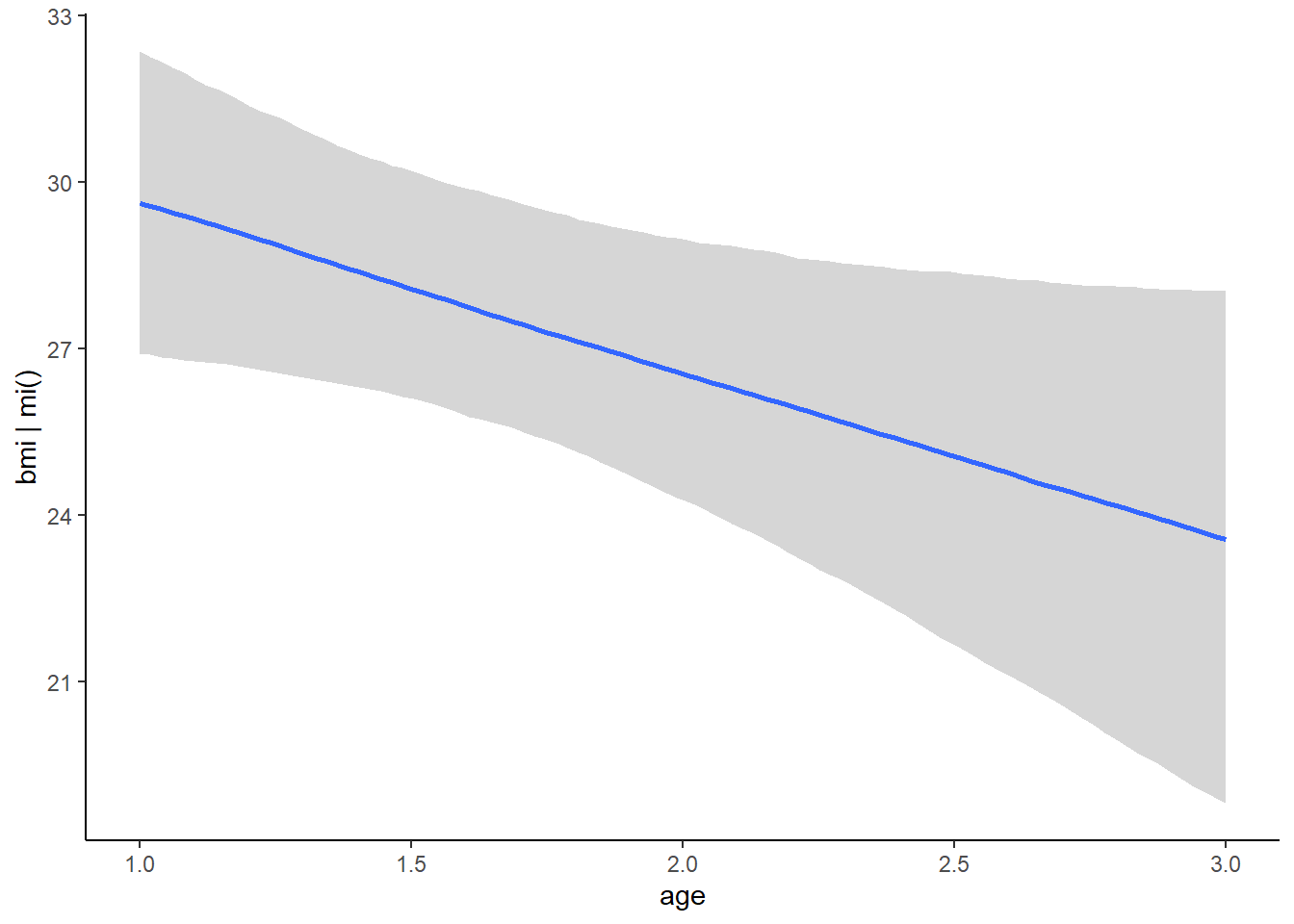
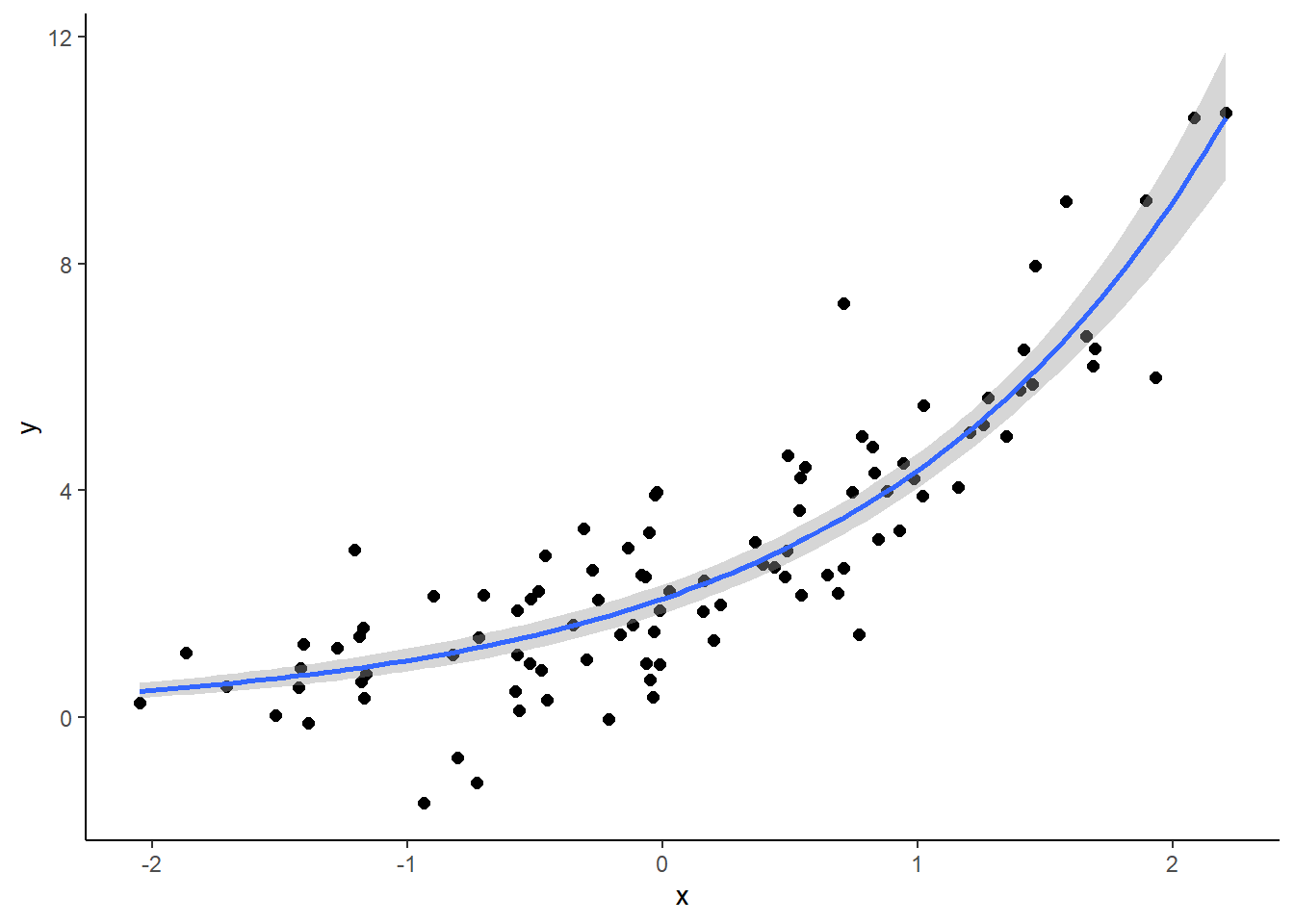
Non-linear models
Non-linear models can also be fit within bf(), you have to specify that the model is non-linear (with nl = TRUE), and also specify the model parameters explicitly. If the model parameters are not dependent upon anything this takes the form of a param ~ 1 section, otherwise it can be a param ~ Variable section. The below example is based upon the example in the non-linear vignette in brms.
set.seed(45276)
b <- c(2, 0.75)
x <- rnorm(100)
y <- rnorm(100, mean = b[1] * exp(b[2] * x))
site <- gl(25,4)
dat1 <- data.frame(x, y, site)
prior1 <- prior(normal(1, 2), nlpar = "b1") +
prior(normal(0, 2), nlpar = "b2")
fit1 <- brm(bf(y ~ b1 * exp(b2 * x), b1 ~ (1|site), b2 ~ 1, nl = TRUE),
data = dat1, prior = prior1, cores = 4,
control = list(adapt_delta = 0.9))
summary(fit1)## Family: gaussian
## Links: mu = identity; sigma = identity
## Formula: y ~ b1 * exp(b2 * x)
## b1 ~ (1 | site)
## b2 ~ 1
## Data: dat1 (Number of observations: 100)
## Samples: 4 chains, each with iter = 2000; warmup = 1000; thin = 1;
## total post-warmup samples = 4000
##
## Group-Level Effects:
## ~site (Number of levels: 25)
## Estimate Est.Error l-95% CI u-95% CI Rhat Bulk_ESS Tail_ESS
## sd(b1_Intercept) 0.09 0.07 0.00 0.25 1.00 2391 2096
##
## Population-Level Effects:
## Estimate Est.Error l-95% CI u-95% CI Rhat Bulk_ESS Tail_ESS
## b1_Intercept 2.09 0.13 1.84 2.34 1.00 3041 2490
## b2_Intercept 0.74 0.04 0.65 0.82 1.00 3138 2481
##
## Family Specific Parameters:
## Estimate Est.Error l-95% CI u-95% CI Rhat Bulk_ESS Tail_ESS
## sigma 1.10 0.08 0.96 1.26 1.00 5510 3180
##
## Samples were drawn using sampling(NUTS). For each parameter, Bulk_ESS
## and Tail_ESS are effective sample size measures, and Rhat is the potential
## scale reduction factor on split chains (at convergence, Rhat = 1).plot(fit1)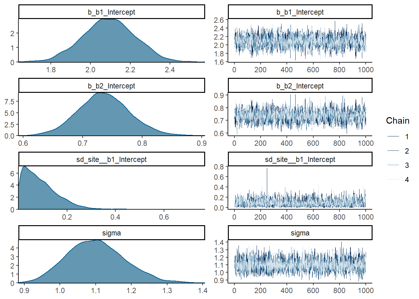
plot(conditional_effects(fit1), points = TRUE)