Analysis of Variance

This tutorial is the second part of the introduction to simple linear regression in R, the use of ANOVAs with categorical predictors.

First we’re going to load in all the packages we’ll be using in this analysis.

library(agridat)          # a package of agricultural datasets
library(summarytools)     # useful functions for summarising datasets
library(dplyr)            # manipulating data
library(ggplot2)          # plotting
library(gridExtra)        # plotting in panels
library(car)              # extensions for regression
library(AICcmodavg)       # calculates AICc

As we’re plotting with ggplot I’m going to set the theme now for the whole tutorial to make it look nicer to me - see the plotting tutorial for more information on the plotting commands.

theme_set(theme_bw() + theme(panel.grid = element_blank()))

We’re going to be using the apples data from the agridat package, an experiment from the 1980s on the impact of spacing, root stock and cultivars on apple tree yields. We’ll be focusing on the impact of spacing, which came in three different treatments: 6m, 10m and 14m apart.

apples <- agridat::archbold.apple
head(apples)

##   rep row pos spacing    stock     gen yield trt
## 1  R1   2   1       6 Seedling Redspur  70.9 601
## 2  R1   2   2       6 Seedling  Golden 130.9 602
## 3  R1   2   8       6    MM111 Redspur 114.5 611
## 4  R1   2   7       6    MM111  Golden  90.5 612
## 5  R1   2   3       6    M0007 Redspur 151.8 671
## 6  R1   2   4       6    M0007  Golden 125.0 672

str(apples)

## 'data.frame':    120 obs. of  8 variables:
##  $ rep    : Factor w/ 5 levels "R1","R2","R3",..: 1 1 1 1 1 1 1 1 1 1 ...
##  $ row    : int  2 2 2 2 2 2 2 2 2 2 ...
##  $ pos    : int  1 2 8 7 3 4 5 6 16 12 ...
##  $ spacing: int  6 6 6 6 6 6 6 6 10 10 ...
##  $ stock  : Factor w/ 4 levels "M0007","MM106",..: 4 4 3 3 1 1 2 2 3 1 ...
##  $ gen    : Factor w/ 2 levels "Golden","Redspur": 2 1 2 1 2 1 2 1 2 2 ...
##  $ yield  : num  70.9 130.9 114.5 90.5 151.8 ...
##  $ trt    : int  601 602 611 612 671 672 661 662 1011 1071 ...

print(dfSummary(apples), method = "render")

Data Frame Summary

apples

Dimensions: 120 x 8
Duplicates: 0

Variable

Stats / Values

Freqs (% of Valid)

Graph

Valid

Missing

rep [factor]

1. R1 2. R2 3. R3 4. R4 5. R5

24	(	20.0%	)
24	(	20.0%	)
24	(	20.0%	)
24	(	20.0%	)
24	(	20.0%	)

120 (100%)

0 (0%)

row [integer]

Mean (sd) : 9 (4.4) min < med < max: 2 < 9 < 16 IQR (CV) : 7.2 (0.5)

15 distinct values

120 (100%)

0 (0%)

pos [integer]

Mean (sd) : 9.2 (4.9) min < med < max: 1 < 10 < 17 IQR (CV) : 9 (0.5)

17 distinct values

120 (100%)

0 (0%)

spacing [integer]

Mean (sd) : 10 (3.3) min < med < max: 6 < 10 < 14 IQR (CV) : 8 (0.3)

6	:	40	(	33.3%	)
10	:	40	(	33.3%	)
14	:	40	(	33.3%	)

120 (100%)

0 (0%)

stock [factor]

1. M0007 2. MM106 3. MM111 4. Seedling

30	(	25.0%	)
30	(	25.0%	)
30	(	25.0%	)
30	(	25.0%	)

120 (100%)

0 (0%)

gen [factor]

1. Golden 2. Redspur

60	(	50.0%	)
60	(	50.0%	)

120 (100%)

0 (0%)

yield [numeric]

Mean (sd) : 145.4 (47.5) min < med < max: 64.1 < 147.1 < 282.3 IQR (CV) : 68.3 (0.3)

85 distinct values

92 (76.67%)

28 (23.33%)

trt [integer]

Mean (sd) : 1036.5 (329.4) min < med < max: 601 < 1036.5 < 1472 IQR (CV) : 735.5 (0.3)

24 distinct values

120 (100%)

0 (0%)

Generated by summarytools 0.9.3 (R version 3.6.0)
2019-05-31

So do apples that are closer together have lower yield? There are only 3 spacing values so we’ll convert it to a categorical variable using as.factor.

apples$spacing2 <- as.factor(apples$spacing)

ggplot(apples, aes(spacing2, yield)) +
    geom_boxplot() +
    labs(x = "Spacing (m)", y = "Yield (kg)")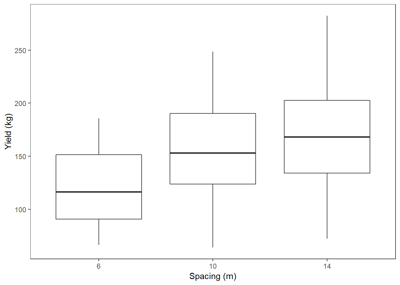

Within R lm and aov give the same result with a single categorical predictor only difference is output of summary functions, which can be changed using summary.lm and summary.aov

now run linear model with lm to see if difference is statistically significant

apples.m <- lm(yield ~ spacing2, data = apples)
summary(apples.m)

## 
## Call:
## lm(formula = yield ~ spacing2, data = apples)
## 
## Residuals:
##     Min      1Q  Median      3Q     Max 
## -92.389 -30.577  -3.516  33.192 117.628 
## 
## Coefficients:
##             Estimate Std. Error t value Pr(>|t|)    
## (Intercept)  120.566      7.382  16.332  < 2e-16 ***
## spacing210    35.924     11.073   3.244 0.001659 ** 
## spacing214    44.107     10.966   4.022 0.000121 ***
## ---
## Signif. codes:  0 '***' 0.001 '**' 0.01 '*' 0.05 '.' 0.1 ' ' 1
## 
## Residual standard error: 43.67 on 89 degrees of freedom
##   (28 observations deleted due to missingness)
## Multiple R-squared:  0.1742, Adjusted R-squared:  0.1556 
## F-statistic: 9.385 on 2 and 89 DF,  p-value: 0.0002003

output gives the difference between the 10m spacing and the 6m spacing, and the 14m spacing and the 6m spacing. The 6m spacing is given by the intercept

use plots to examine residuals.

par(mfrow=c(2,2));plot(apples.m);par(mfrow=c(1,1))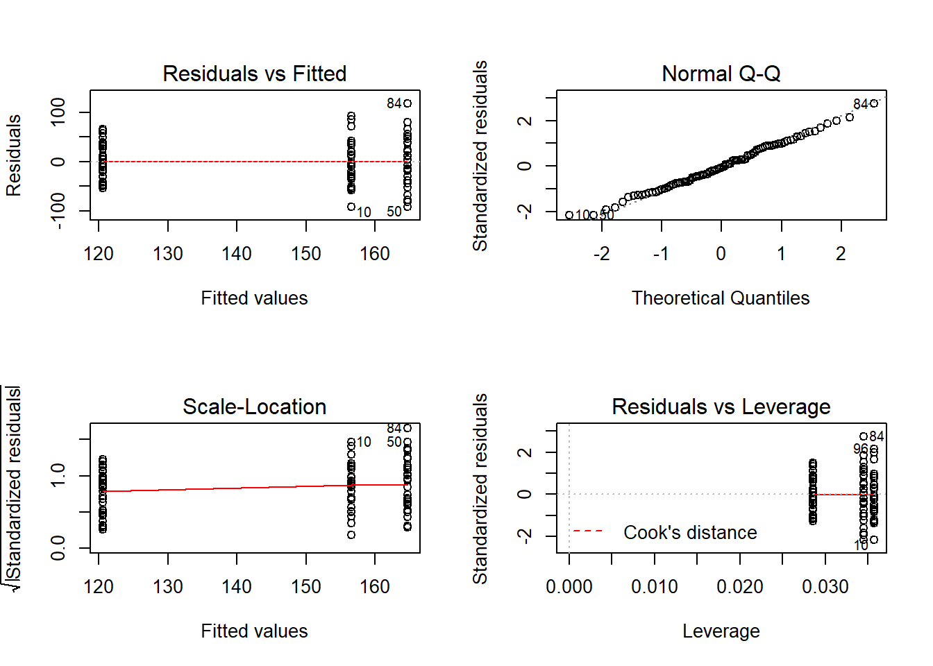

qqp(apples.m)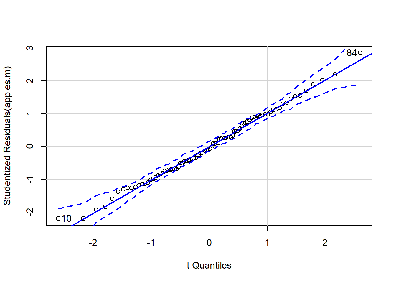

## [1] 10 84

If wish to do a Tukey’s HSD post-hoc test then need to fit model with aov rather than lm

apples.aov <- aov(yield ~ spacing2, data = apples)
summary(apples.aov)

##             Df Sum Sq Mean Sq F value Pr(>F)    
## spacing2     2  35801   17900   9.385  2e-04 ***
## Residuals   89 169750    1907                   
## ---
## Signif. codes:  0 '***' 0.001 '**' 0.01 '*' 0.05 '.' 0.1 ' ' 1
## 28 observations deleted due to missingness

summary(apples.m) # compare to lm output - different format but same numbers

## 
## Call:
## lm(formula = yield ~ spacing2, data = apples)
## 
## Residuals:
##     Min      1Q  Median      3Q     Max 
## -92.389 -30.577  -3.516  33.192 117.628 
## 
## Coefficients:
##             Estimate Std. Error t value Pr(>|t|)    
## (Intercept)  120.566      7.382  16.332  < 2e-16 ***
## spacing210    35.924     11.073   3.244 0.001659 ** 
## spacing214    44.107     10.966   4.022 0.000121 ***
## ---
## Signif. codes:  0 '***' 0.001 '**' 0.01 '*' 0.05 '.' 0.1 ' ' 1
## 
## Residual standard error: 43.67 on 89 degrees of freedom
##   (28 observations deleted due to missingness)
## Multiple R-squared:  0.1742, Adjusted R-squared:  0.1556 
## F-statistic: 9.385 on 2 and 89 DF,  p-value: 0.0002003

summary.lm(apples.aov) # can get equivalent output to lm using summary.lm

## 
## Call:
## aov(formula = yield ~ spacing2, data = apples)
## 
## Residuals:
##     Min      1Q  Median      3Q     Max 
## -92.389 -30.577  -3.516  33.192 117.628 
## 
## Coefficients:
##             Estimate Std. Error t value Pr(>|t|)    
## (Intercept)  120.566      7.382  16.332  < 2e-16 ***
## spacing210    35.924     11.073   3.244 0.001659 ** 
## spacing214    44.107     10.966   4.022 0.000121 ***
## ---
## Signif. codes:  0 '***' 0.001 '**' 0.01 '*' 0.05 '.' 0.1 ' ' 1
## 
## Residual standard error: 43.67 on 89 degrees of freedom
##   (28 observations deleted due to missingness)
## Multiple R-squared:  0.1742, Adjusted R-squared:  0.1556 
## F-statistic: 9.385 on 2 and 89 DF,  p-value: 0.0002003

TukeyHSD(apples.aov)

##   Tukey multiple comparisons of means
##     95% family-wise confidence level
## 
## Fit: aov(formula = yield ~ spacing2, data = apples)
## 
## $spacing2
##            diff        lwr      upr     p adj
## 10-6  35.923571   9.530402 62.31674 0.0046832
## 14-6  44.106700  17.967561 70.24584 0.0003526
## 14-10  8.183128 -19.396838 35.76309 0.7598733

ANOVA with unbalanced designs and > 1 predictor

Balanced designs have the same number of reps per treatment. This is often not the case, and the study is unbalanced. If the study is unbalanced the way in which predictors are evaluated impacts the result. The different ways of evaluating predictors are known as Type I, Type II and Type III ANOVAs

To find out more about this go to http://goanna.cs.rmit.edu.au/~fscholer/anova.php

For type III tests to be correct need to change the way R codes factors

options(contrasts = c("contr.sum", "contr.poly"))

This won’t change type I or II Default is: options(contrasts = c(“contr.treatment”, “contr.poly”))

A        = c("a", "a", "a", "a", "b", "b", "b", "b", "b", "b", "b", "b")
B        = c("x", "y", "x", "y", "x", "y", "x", "y", "x", "x", "x", "x")
C        = c("l", "l", "m", "m", "l", "l", "m", "m", "l", "l", "l", "l")
response = c( 14,  30,  15,  35,  50,  51,  30,  32,  51,  55,  53,  55)

model = lm(response ~ A + B + C + A:B + A:C + B:C)

anova(model)              # Type I tests

## Analysis of Variance Table
## 
## Response: response
##           Df  Sum Sq Mean Sq  F value    Pr(>F)    
## A          1 1488.37 1488.37 357.6869 7.614e-06 ***
## B          1   18.22   18.22   4.3798 0.0905765 .  
## C          1  390.15  390.15  93.7610 0.0001995 ***
## A:B        1  278.68  278.68  66.9722 0.0004431 ***
## A:C        1  339.51  339.51  81.5909 0.0002778 ***
## B:C        1    8.51    8.51   2.0444 0.2121592    
## Residuals  5   20.81    4.16                       
## ---
## Signif. codes:  0 '***' 0.001 '**' 0.01 '*' 0.05 '.' 0.1 ' ' 1

Anova(model, type="II")   # Type II tests using car package

## Anova Table (Type II tests)
## 
## Response: response
##            Sum Sq Df  F value    Pr(>F)    
## A         1022.01  1 245.6103 1.923e-05 ***
## B          131.25  1  31.5421 0.0024764 ** 
## C          278.68  1  66.9722 0.0004431 ***
## A:B        180.01  1  43.2593 0.0012194 ** 
## A:C        321.01  1  77.1445 0.0003174 ***
## B:C          8.51  1   2.0444 0.2121592    
## Residuals   20.81  5                       
## ---
## Signif. codes:  0 '***' 0.001 '**' 0.01 '*' 0.05 '.' 0.1 ' ' 1

Anova(model, type="III")  # Type III tests using car package

## Anova Table (Type III tests)
## 
## Response: response
##             Sum Sq Df   F value    Pr(>F)    
## (Intercept) 9490.0  1 2280.6425 7.605e-08 ***
## A            724.5  1  174.1138 4.465e-05 ***
## B            184.5  1   44.3408 0.0011526 ** 
## C            180.0  1   43.2593 0.0012194 ** 
## A:B          180.0  1   43.2593 0.0012194 ** 
## A:C          321.0  1   77.1445 0.0003174 ***
## B:C            8.5  1    2.0444 0.2121592    
## Residuals     20.8  5                        
## ---
## Signif. codes:  0 '***' 0.001 '**' 0.01 '*' 0.05 '.' 0.1 ' ' 1

Balanced design shows no difference between type I, II and III

A        = c("a", "a", "a", "a", "a", "a", "b", "b", "b", "b", "b", "b")
B        = c("x", "y", "x", "y", "x", "y", "x", "y", "x", "y", "x", "y")
C        = c("l", "l", "m", "m", "l", "l", "m", "m", "l", "l", "m", "m")
response = c( 14,  30,  15,  35,  50,  51,  30,  32,  51,  55,  53,  55)

model = lm(response ~ A + B + C + A:B + A:C + B:C)

anova(model)              # Type I tests

## Analysis of Variance Table
## 
## Response: response
##           Df  Sum Sq Mean Sq F value Pr(>F)
## A          1  546.75  546.75  1.9146 0.2250
## B          1  168.75  168.75  0.5909 0.4768
## C          1  315.38  315.38  1.1044 0.3414
## A:B        1   70.08   70.08  0.2454 0.6413
## A:C        1    0.38    0.38  0.0013 0.9725
## B:C        1   15.04   15.04  0.0527 0.8276
## Residuals  5 1427.87  285.57

Anova(model, type="II")   # Type II tests

## Anova Table (Type II tests)
## 
## Response: response
##            Sum Sq Df F value Pr(>F)
## A          782.04  1  2.7385 0.1589
## B          168.75  1  0.5909 0.4768
## C          315.38  1  1.1044 0.3414
## A:B         84.37  1  0.2955 0.6101
## A:C          0.38  1  0.0013 0.9725
## B:C         15.04  1  0.0527 0.8276
## Residuals 1427.87  5

Anova(model, type="III")  # Type III tests

## Anova Table (Type III tests)
## 
## Response: response
##              Sum Sq Df F value    Pr(>F)    
## (Intercept) 16380.4  1 57.3593 0.0006367 ***
## A             782.0  1  2.7385 0.1588624    
## B             168.7  1  0.5909 0.4767865    
## C             315.4  1  1.1044 0.3414277    
## A:B            84.4  1  0.2955 0.6100929    
## A:C             0.4  1  0.0013 0.9724954    
## B:C            15.0  1  0.0527 0.8275710    
## Residuals    1427.9  5                      
## ---
## Signif. codes:  0 '***' 0.001 '**' 0.01 '*' 0.05 '.' 0.1 ' ' 1

The choice between the types of ANOVAs is beyond the scope of this R club and is hypothesis dependent.

Last updated on 28 Mar, 2018