This is a continuation of the tutorial on data manipulation, with many examples of different summary tables and statistics. It’s largely using the janitor, summarytools and psych packages which have loads of great functions for quickly examining your data and I highly recommend them!
First of all we need to load up the packages we want to use today
library(readr)   ## for reading in data
library(dplyr)   ## for data manipulation
library(janitor) ## for data cleaning tools
library(psych)   ## for some useful data exploration graphs
library(summarytools) ## for some summary statistics and tables
We’re using the same data as the data manipulation tutorial to show a variety of different summary statistics and tables
CS <- read_csv("CS_fake.csv")
CS <- clean_names(CS)
CS
## # A tibble: 1,000 x 7
## plot_id country county carbon_percent nitrogen_percent ph habitat
## <chr> <chr> <chr> <dbl> <dbl> <dbl> <dbl>
## 1 GCEXWQRY~ VAL ERROLD 70.2 7.70 2.85 8
## 2 JZCMAHEP~ RET BOLTHAV~ 14.5 1.53 6.04 7
## 3 DTVGQBSJ~ VAL TREVALE 28.6 5.93 5.00 4
## 4 REJAJMVE~ HAR GREENVA~ 24.0 1.64 5.43 2
## 5 FMWEYMKI~ VAL EVENDIM 14.9 2.84 6.85 8
## 6 KYULXCMW~ VAL EVENDIM 57.8 6.89 3.17 6
## 7 CPKKYGMV~ RET PETRAS 33.3 4.53 4.55 7
## 8 TAYSUFTD~ RET PETRAS 56.0 8.01 3.05 5
## 9 EAYSCYXE~ VAL ERROLD 12.3 5.18 5.97 6
## 10 NZONLIZV~ VAL EVENDIM 74.5 10.0 2.54 9
## # ... with 990 more rowsSummary tables and statistics
There’s a lot of different functions in R for summarising dataframes, so we’re going to go through a few useful ones
The summarytools package has a few useful functions, such as the summary table produced below:
print(dfSummary(CS[,2:6], style = 'grid', graph.magnif = 0.85), method = "render", omit.headings = TRUE)| No | Variable | Stats / Values | Freqs (% of Valid) | Graph | Valid | Missing | ||||||||||||||||||||||||||||
|---|---|---|---|---|---|---|---|---|---|---|---|---|---|---|---|---|---|---|---|---|---|---|---|---|---|---|---|---|---|---|---|---|---|---|
| 1 | country [character] | 1. HAR 2. RET 3. VAL |
|
 |
1000 (100%) | 0 (0%) | ||||||||||||||||||||||||||||
| 2 | county [character] | 1. BERRYFORD 2. BOLTHAVEN 3. ERROLD 4. EVENDIM 5. GREENVALE 6. PETRAS 7. TREVALE |
|
 |
1000 (100%) | 0 (0%) | ||||||||||||||||||||||||||||
| 3 | carbon_percent [numeric] | Mean (sd) : 34.9 (16.4) min < med < max: 4.4 < 31.3 < 105.2 IQR (CV) : 20.3 (0.5) | 998 distinct values |  |
999 (99.9%) | 1 (0.1%) | ||||||||||||||||||||||||||||
| 4 | nitrogen_percent [numeric] | Mean (sd) : 4.8 (2) min < med < max: 0 < 4.6 < 12.7 IQR (CV) : 2.7 (0.4) | 992 distinct values |  |
996 (99.6%) | 4 (0.4%) | ||||||||||||||||||||||||||||
| 5 | ph [numeric] | Mean (sd) : 4.5 (1) min < med < max: 1.5 < 4.5 < 7.5 IQR (CV) : 1.3 (0.2) | 998 distinct values |  |
999 (99.9%) | 1 (0.1%) |
Generated by summarytools 0.9.3 (R version 3.6.0)
2019-05-31
Frequency tables and cross-tabulating factors
Both janitor and summarytools offer functions for frequency tables and cross-tabulating factors.
freq(CS$habitat, style = "rmarkdown", omit.headings = TRUE) ##summarytools| Freq | % Valid | % Valid Cum. | % Total | % Total Cum. | |
|---|---|---|---|---|---|
| 1 | 95 | 9.50 | 9.50 | 9.50 | 9.50 |
| 2 | 107 | 10.70 | 20.20 | 10.70 | 20.20 |
| 3 | 95 | 9.50 | 29.70 | 9.50 | 29.70 |
| 4 | 109 | 10.90 | 40.60 | 10.90 | 40.60 |
| 5 | 106 | 10.60 | 51.20 | 10.60 | 51.20 |
| 6 | 99 | 9.90 | 61.10 | 9.90 | 61.10 |
| 7 | 106 | 10.60 | 71.70 | 10.60 | 71.70 |
| 8 | 99 | 9.90 | 81.60 | 9.90 | 81.60 |
| 9 | 105 | 10.50 | 92.10 | 10.50 | 92.10 |
| 10 | 79 | 7.90 | 100.00 | 7.90 | 100.00 |
| <NA> | 0 | 0.00 | 100.00 | ||
| Total | 1000 | 100.00 | 100.00 | 100.00 | 100.00 |
print(ctable(CS$country, CS$county, prop = "n"), method = "render", omit.headings = TRUE) ##summarytools| county | ||||||||
|---|---|---|---|---|---|---|---|---|
| country | BERRYFORD | BOLTHAVEN | ERROLD | EVENDIM | GREENVALE | PETRAS | TREVALE | Total |
| HAR | 113 | 0 | 0 | 0 | 91 | 0 | 0 | 204 |
| RET | 0 | 165 | 0 | 0 | 0 | 146 | 0 | 311 |
| VAL | 0 | 0 | 156 | 185 | 0 | 0 | 144 | 485 |
| Total | 113 | 165 | 156 | 185 | 91 | 146 | 144 | 1000 |
Generated by summarytools 0.9.3 (R version 3.6.0)
2019-05-31
For me janitor is a little more intuitive, and is also built to be compatible with the pipe operator
tabyl(CS, habitat)## habitat n percent
## 1 95 0.095
## 2 107 0.107
## 3 95 0.095
## 4 109 0.109
## 5 106 0.106
## 6 99 0.099
## 7 106 0.106
## 8 99 0.099
## 9 105 0.105
## 10 79 0.079tabyl(CS, country, county) ## country BERRYFORD BOLTHAVEN ERROLD EVENDIM GREENVALE PETRAS TREVALE
## HAR 113 0 0 0 91 0 0
## RET 0 165 0 0 0 146 0
## VAL 0 0 156 185 0 0 144tabyl(CS, country, habitat, county)## $BERRYFORD
## country 1 2 3 4 5 6 7 8 9 10
## HAR 10 14 9 12 10 9 12 13 17 7
## RET 0 0 0 0 0 0 0 0 0 0
## VAL 0 0 0 0 0 0 0 0 0 0
##
## $BOLTHAVEN
## country 1 2 3 4 5 6 7 8 9 10
## HAR 0 0 0 0 0 0 0 0 0 0
## RET 17 16 19 16 20 13 20 15 14 15
## VAL 0 0 0 0 0 0 0 0 0 0
##
## $ERROLD
## country 1 2 3 4 5 6 7 8 9 10
## HAR 0 0 0 0 0 0 0 0 0 0
## RET 0 0 0 0 0 0 0 0 0 0
## VAL 16 16 12 18 17 17 15 20 15 10
##
## $EVENDIM
## country 1 2 3 4 5 6 7 8 9 10
## HAR 0 0 0 0 0 0 0 0 0 0
## RET 0 0 0 0 0 0 0 0 0 0
## VAL 16 16 22 20 24 11 15 20 22 19
##
## $GREENVALE
## country 1 2 3 4 5 6 7 8 9 10
## HAR 11 14 16 6 4 16 8 4 6 6
## RET 0 0 0 0 0 0 0 0 0 0
## VAL 0 0 0 0 0 0 0 0 0 0
##
## $PETRAS
## country 1 2 3 4 5 6 7 8 9 10
## HAR 0 0 0 0 0 0 0 0 0 0
## RET 12 15 9 17 18 12 21 7 18 17
## VAL 0 0 0 0 0 0 0 0 0 0
##
## $TREVALE
## country 1 2 3 4 5 6 7 8 9 10
## HAR 0 0 0 0 0 0 0 0 0 0
## RET 0 0 0 0 0 0 0 0 0 0
## VAL 13 16 8 20 13 21 15 20 13 5Summary statistics by groups
dataframes can be described by a categorical variable within both summarytools and psych. The describeBy function in psych is simple to write but only likes numeric variables. I also don’t know of any way to pick and choose which stats are reported.
describeBy(CS, "country")##
## Descriptive statistics by group
## country: HAR
## vars n mean sd median trimmed mad min max
## plot_id* 1 204 NaN NA NA NaN NA Inf -Inf
## country* 2 204 NaN NA NA NaN NA Inf -Inf
## county* 3 204 NaN NA NA NaN NA Inf -Inf
## carbon_percent 4 203 34.28 16.07 31.09 32.43 14.31 8.97 98.90
## nitrogen_percent 5 202 3.49 1.93 3.26 3.34 1.82 0.02 10.33
## ph 6 204 4.52 0.99 4.56 4.52 0.91 1.63 6.98
## habitat 7 204 5.18 2.85 5.00 5.15 3.71 1.00 10.00
## range skew kurtosis se
## plot_id* -Inf NA NA NA
## country* -Inf NA NA NA
## county* -Inf NA NA NA
## carbon_percent 89.93 1.29 2.19 1.13
## nitrogen_percent 10.31 0.80 0.83 0.14
## ph 5.35 -0.09 0.19 0.07
## habitat 9.00 0.11 -1.29 0.20
## --------------------------------------------------------
## country: RET
## vars n mean sd median trimmed mad min max
## plot_id* 1 311 NaN NA NA NaN NA Inf -Inf
## country* 2 311 NaN NA NA NaN NA Inf -Inf
## county* 3 311 NaN NA NA NaN NA Inf -Inf
## carbon_percent 4 311 35.36 16.73 32.57 33.59 15.08 7.23 95.20
## nitrogen_percent 5 310 4.55 1.93 4.28 4.45 1.83 0.02 10.62
## ph 6 311 4.46 1.02 4.49 4.47 1.03 1.72 7.53
## habitat 7 311 5.52 2.84 5.00 5.52 2.97 1.00 10.00
## range skew kurtosis se
## plot_id* -Inf NA NA NA
## country* -Inf NA NA NA
## county* -Inf NA NA NA
## carbon_percent 87.97 1.03 1.09 0.95
## nitrogen_percent 10.60 0.50 0.17 0.11
## ph 5.81 -0.08 -0.14 0.06
## habitat 9.00 0.01 -1.18 0.16
## --------------------------------------------------------
## country: VAL
## vars n mean sd median trimmed mad min max
## plot_id* 1 485 NaN NA NA NaN NA Inf -Inf
## country* 2 485 NaN NA NA NaN NA Inf -Inf
## county* 3 485 NaN NA NA NaN NA Inf -Inf
## carbon_percent 4 485 34.80 16.36 31.34 33.14 13.93 4.42 105.24
## nitrogen_percent 5 484 5.43 1.89 5.26 5.31 1.88 1.07 12.71
## ph 6 484 4.49 1.00 4.52 4.50 0.98 1.53 7.29
## habitat 7 485 5.46 2.76 5.00 5.48 2.97 1.00 10.00
## range skew kurtosis se
## plot_id* -Inf NA NA NA
## country* -Inf NA NA NA
## county* -Inf NA NA NA
## carbon_percent 100.82 1.18 2.02 0.74
## nitrogen_percent 11.64 0.72 0.87 0.09
## ph 5.76 -0.11 0.09 0.05
## habitat 9.00 -0.02 -1.18 0.13summarytools’ version is longer to write but appears to be more flexible. I’ve set some parameters here to make it print better on this document - you may want to remove the style and method arguments to make it look nicer when working from the console.
## summarytools's version is longer to write but more flexible
# First save the results
CS_stats_by_country <- by(data = CS,
                          INDICES = CS$country,
                          FUN = descr, stats = c("mean", "sd", "min", "med", "max"),
                          transpose = TRUE, style = "rmarkdown", omit.headings = TRUE)
# then view
view(CS_stats_by_country, method = "pander")
Group: country = HAR
| Mean | Std.Dev | Min | Median | Max | |
|---|---|---|---|---|---|
| carbon_percent | 34.28 | 16.07 | 8.97 | 31.09 | 98.90 |
| habitat | 5.18 | 2.85 | 1.00 | 5.00 | 10.00 |
| nitrogen_percent | 3.49 | 1.93 | 0.02 | 3.26 | 10.33 |
| ph | 4.52 | 0.99 | 1.63 | 4.56 | 6.98 |
Group: country = RET
| Mean | Std.Dev | Min | Median | Max | |
|---|---|---|---|---|---|
| carbon_percent | 35.36 | 16.73 | 7.23 | 32.57 | 95.20 |
| habitat | 5.52 | 2.84 | 1.00 | 5.00 | 10.00 |
| nitrogen_percent | 4.55 | 1.93 | 0.02 | 4.28 | 10.62 |
| ph | 4.46 | 1.02 | 1.72 | 4.49 | 7.53 |
Group: country = VAL
| Mean | Std.Dev | Min | Median | Max | |
|---|---|---|---|---|---|
| carbon_percent | 34.80 | 16.36 | 4.42 | 31.34 | 105.24 |
| habitat | 5.46 | 2.76 | 1.00 | 5.00 | 10.00 |
| nitrogen_percent | 5.43 | 1.89 | 1.07 | 5.26 | 12.71 |
| ph | 4.49 | 1.00 | 1.53 | 4.52 | 7.29 |
You can do the above using group_by() then summarise() from the dplyr package but as far as I know you’ll have to manually write out which stats you want which can be a hassle:
CS %>% group_by(country) %>%
  summarise(mean_pH = mean(ph, na.rm = TRUE),
            mean_carbon = mean(carbon_percent, na.rm = TRUE))
## # A tibble: 3 x 3
## country mean_pH mean_carbon
## <chr> <dbl> <dbl>
## 1 HAR 4.52 34.3
## 2 RET 4.46 35.4
## 3 VAL 4.49 34.8Quick graphs
While summary statistic tables can be very useful they are no substitute for plotting out your data. For an interesting discussion about this (with dinosaurs!) see this page on how different datasets can be with the same summary statistics.
Histograms are great for seeing what kind of distributions your variables have, I often use the multi.hist function from within the psych package to look at my data quickly and easily. Note that this function doesn’t always return the plotting environment to what it was previously so we specify that the plotting parameters should return to one plot per page afterwards
multi.hist(CS[,4:6])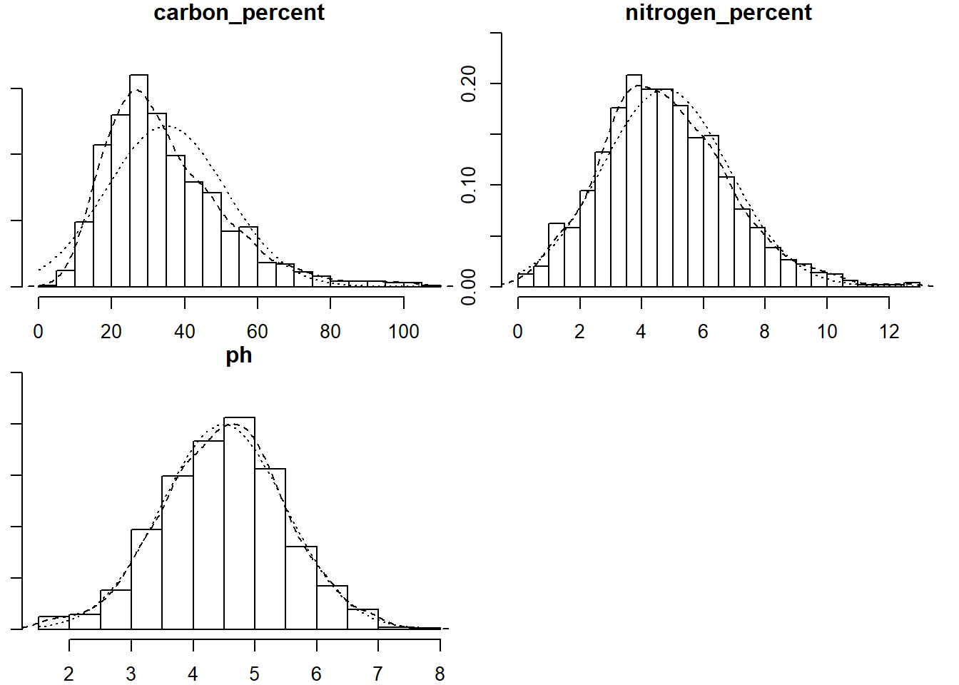
par(mfrow=c(1,1)) The pairs plot within R, and the extensions upon it from many other package, is a great way to see how the variables from your dataset are related to each other.The pairs.panels function in psych shows the name of each variable and its histogram down the diagonal, the scatterplots on the lower triangle and the correlation coefficient on the upper triangle. You can change the type of correlation coefficient, and various plotting parameters easily.
pairs.panels(CS[,4:6])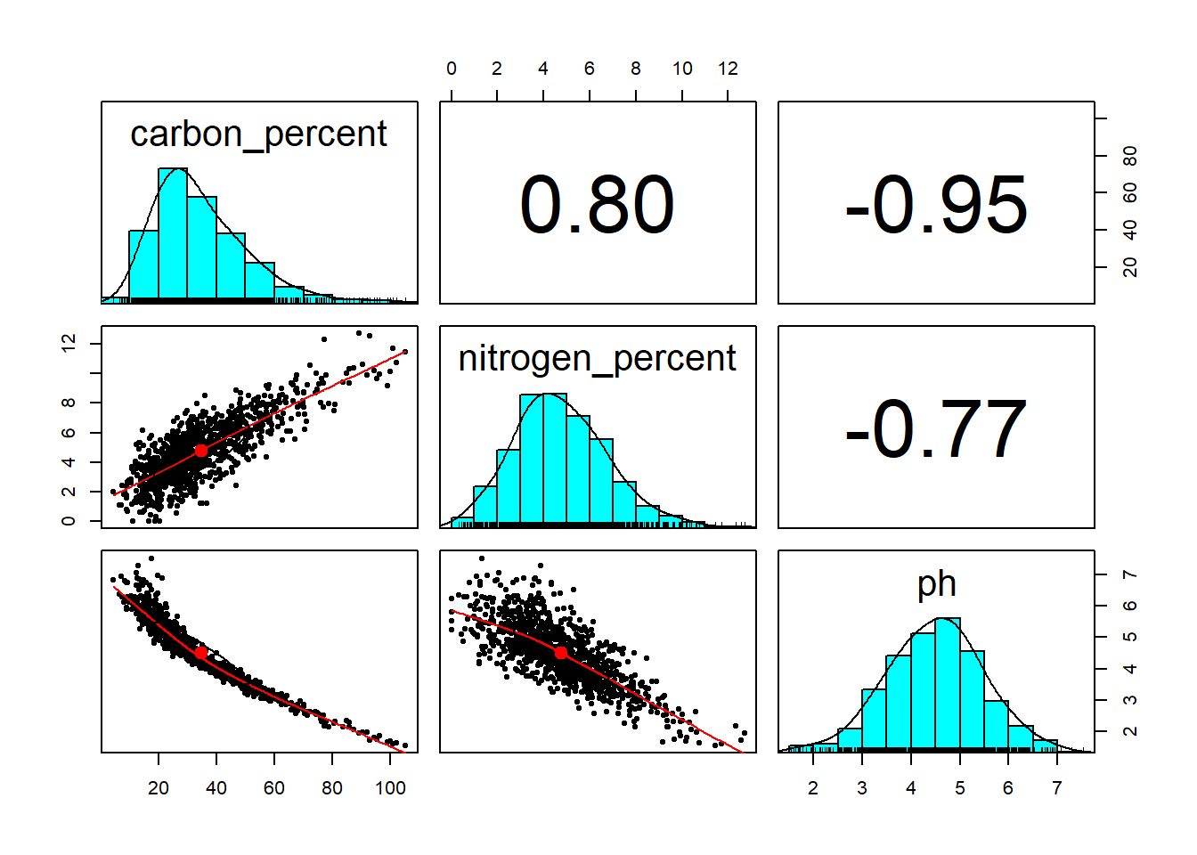
If you want to take an in depth look at one of the plots and identify certain points then you can plot the scatterplot and use the identify function to interactively select points and get a label for what they are - this doesn’t work in rmarkdown but you can try it yourself.
plot(nitrogen_percent ~ carbon_percent, CS)
identify(CS$carbon_percent, CS$nitrogen_percent, labels=CS$plot_id)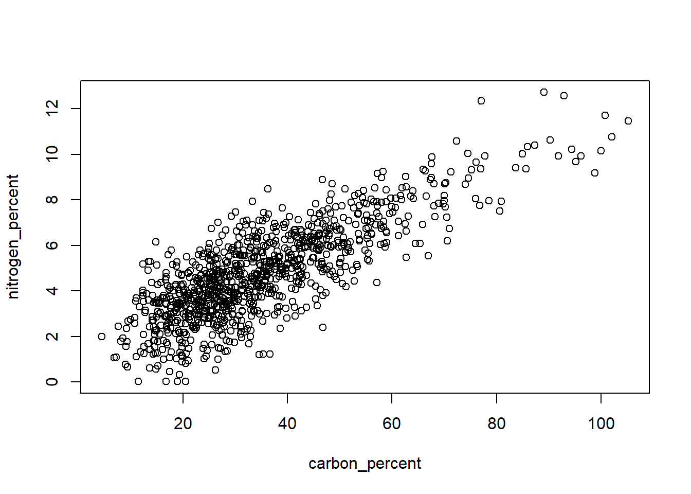
Other useful plots include coplots in base R, which show how the relationship between two variables changes with a third variable
coplot(ph ~ carbon_percent|nitrogen_percent, CS)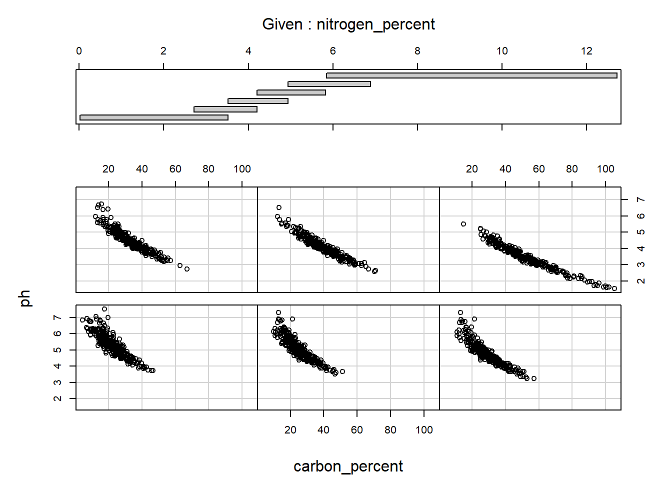
That’s all that comes to mind right now. There are so many different ways of manipulating and exploring datasets in R. These are just a few that I have found useful and I hope you do too!