In R there are multiple ways to combine plots together into one mega-plot. We’ll first briefly go through a couple of ways using base R functions and then compare methods for combining ggplot2 plots into mega-plots. We’ll be mainly using the cowplot and egg packages, and a lot of this is based off the vignettes for those which can be found at the links specified.
Base R functions for panel plots
The simplest way to combine multiple plots into one in base R is to change the graphical parameters so that instead of starting a new page each time you plot a new plot you add it to the next slot in the current page. You can change the number of slots in each page by changing the mfrow value in par.
data(iris)
par(mfrow = c(1, 2)) # here we set the new number of rows of plots to be 1 and the number of columns to two
hist(iris$Sepal.Length)
hist(iris$Petal.Length)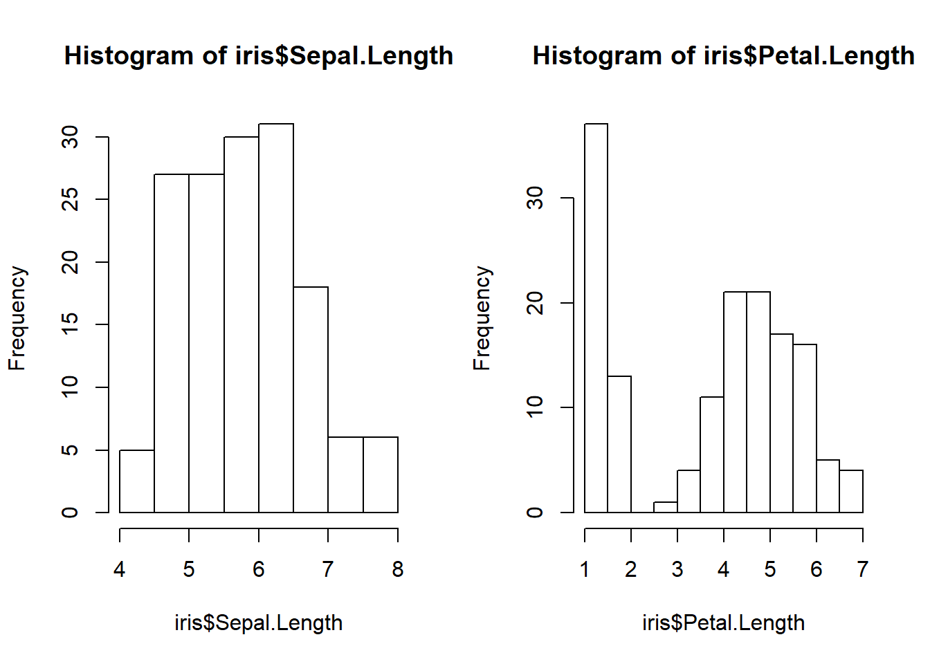
It’s generally a good idea to set mfrow back again to c(1,1) once you have finished as it will stay at whatever you have it currently for the rest of the session (this has caught me out many many times).
par(mfrow = c(1,1))There is no limit to how many rows and columns you can choose by changing mfrow but it will always result in every plot taking up the same size of space. If you want one plot to be bigger than the others you are better off using the layout function. Here you give layout a matrix that explains how you want the plots laid out on the page. We build a matrix using the matrix function, saying that we want 2 rows, 2 columns, for the first two plots to take up one unit and for the third to take up two units of space.
layout(matrix(c(1,2,3,3),nrow=2,ncol = 2, byrow = TRUE))
hist(iris$Sepal.Length)
hist(iris$Petal.Length)
plot(Sepal.Length ~ Petal.Length, iris)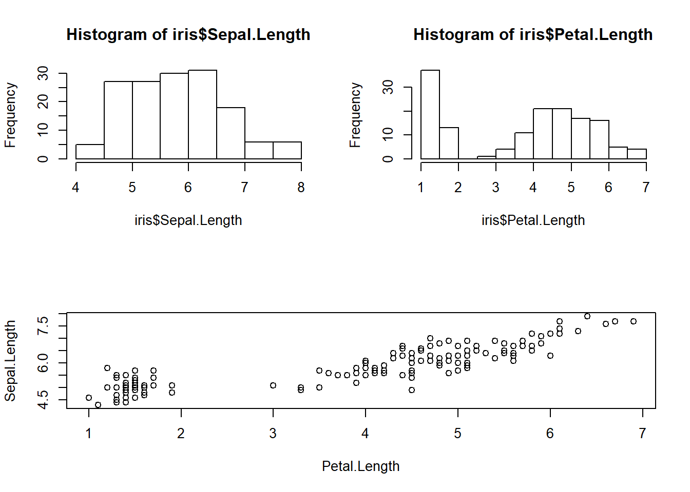
par(mfrow=c(1,1))Multiple plots with ggplots
There are numerous packages that take ggplot2 objects and can combine them into multiple plots. The gridExtra package has been around the longest, but I’m going to focus on the cowplot and the egg packages in this tutorial as they have useful functionality regarding alignment of plots.
The cowplot package has the plot_grid function which will combine plots into one - this does not automatically align the plot content though.
require(cowplot)

plot.mpg <- ggplot(mpg, aes(x = cty, y = hwy, colour = factor(cyl))) +
  geom_point(size=2.5)
plot.diamonds <- ggplot(diamonds, aes(clarity, fill = cut)) + geom_bar() +
  theme(axis.text.x = element_text(angle=70, vjust=0.5))

plot_grid(plot.mpg, plot.diamonds, labels = c('A', 'B'))
To align the plot contents you add an argument stating that align = “h” for horizontally, “v” for vertically or “hv” for both.
plot_grid(plot.mpg, plot.diamonds, align = "h", labels = c('A', 'B'))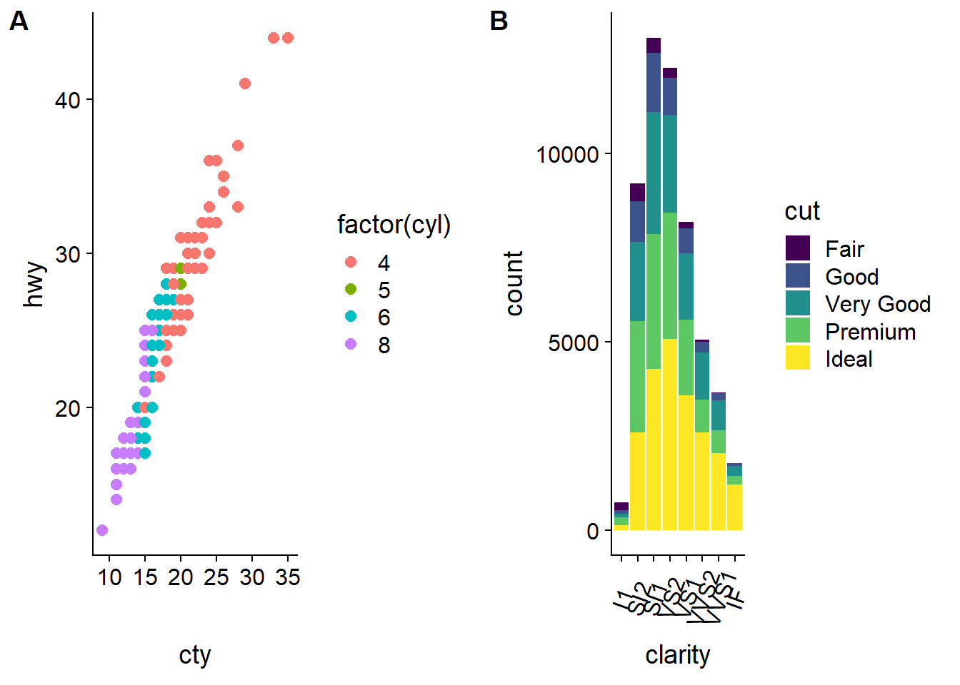
The egg package, by contrast, automatically aligns plots within its ggarrange function:
require(egg)
ggarrange(plot.mpg, plot.diamonds, nrow = 1, labels = c("A","B"))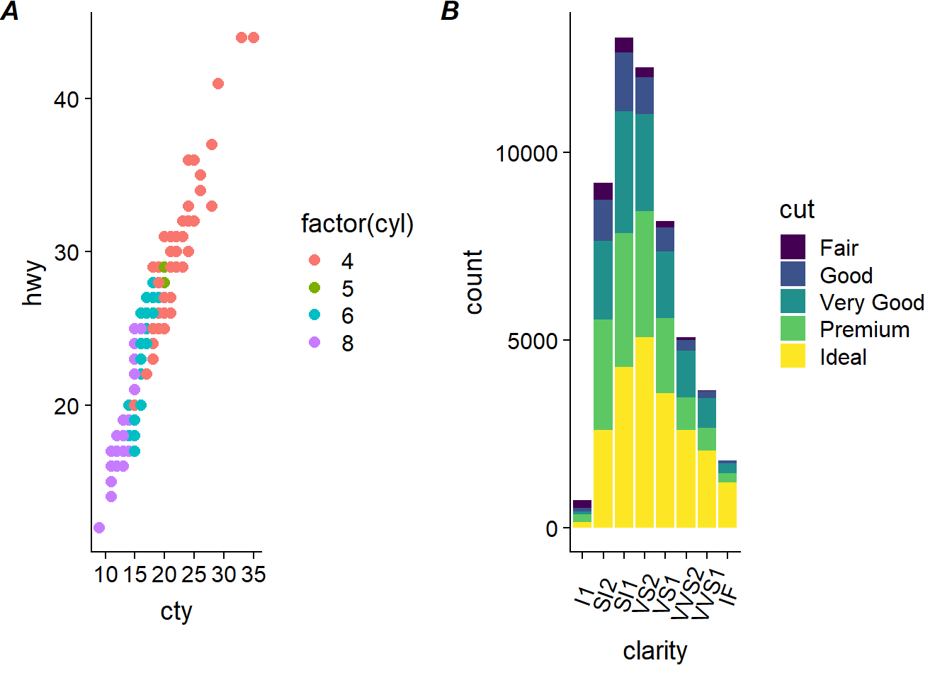
As an aside, grid.arrange from the gridExtra package is much more difficult to get the plots to align in. You have to modify the ggtable objects given to the grid.arrange function directly.
Complex layouts
Often we don’t want a simple grid but instead want one plot to be larger than the others, there are a couple of ways to do this as well.
Changing relative size of plots
If you just want to change the relative size of plots within the grid egg and cowplot have simple arguments to ggarrange and plot_grid respectively that change the ratio of plots.
plot.iris <- ggplot(iris, aes(Sepal.Length, Sepal.Width)) +
  geom_point() + facet_grid(. ~ Species) + stat_smooth(method = "lm") +
  background_grid(major = 'y', minor = "none") + # add thin horizontal lines
  panel_border() # and a border around each panel

ggarrange(plot.mpg, plot.diamonds, plot.iris, widths = c(5, 1), heights = c(3, 1))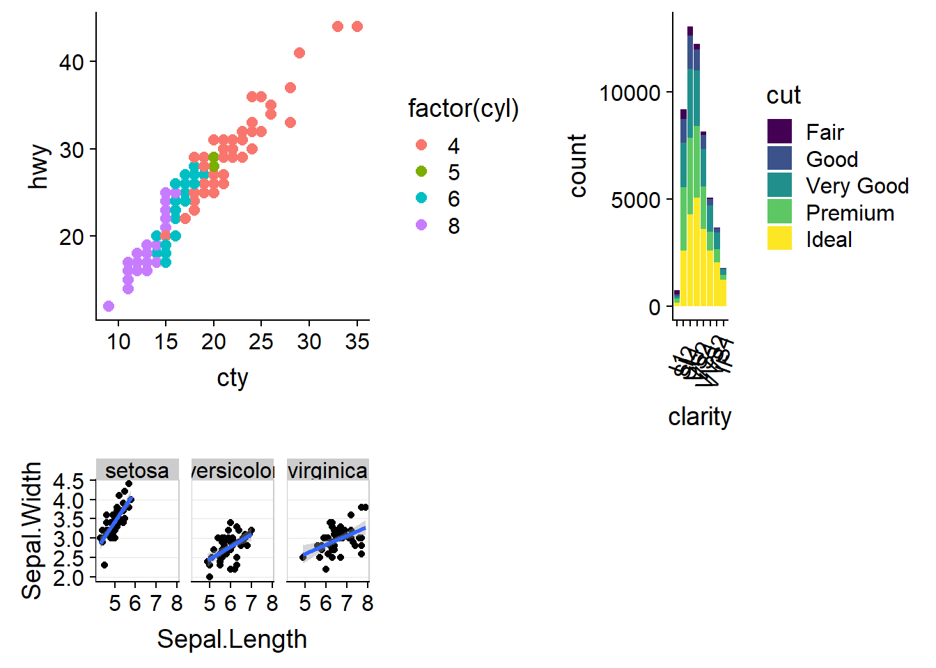
plot_grid(plot.mpg, plot.diamonds, plot.iris, rel_widths = c(1.5, 1), rel_heights = c(2, 1))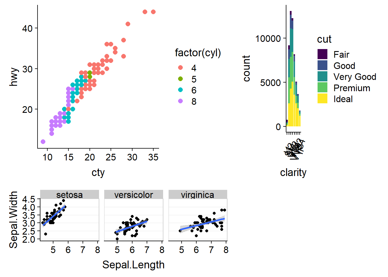
Note that cowplot and egg calculate the ratio of height and width differently so the numbers to get the same effect are different.
Nested layouts
If we want one plot to cover multiple slots within the panel it is a little more complicated, but possible for both. Within cowplot we nest together two layouts:
bottom_row <- plot_grid(plot.mpg, plot.diamonds, labels = c('B', 'C'), align = 'h', rel_widths = c(1, 1.3))
plot_grid(plot.iris, bottom_row, labels = c('A', ''), ncol = 1, rel_heights = c(1, 1.2))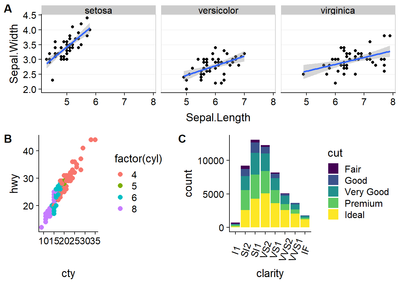
These can be aligned using the align_plots() function:
# first align the top-row plot (plot.iris) with the left-most plot of the
# bottom row (plot.mpg)
plots <- align_plots(plot.mpg, plot.iris, align = 'v', axis = 'l')
# then build the bottom row
bottom_row <- plot_grid(plots[[1]], plot.diamonds,
                        labels = c('B', 'C'), align = 'h', rel_widths = c(1, 1.3))
# then combine with the top row for final plot
plot_grid(plots[[2]], bottom_row, labels = c('A', ''), ncol = 1, rel_heights = c(1, 1.2))
Within egg you first get the grid graphical object (or grob) from each plot, then convert into a 3x3 gtable with the central cell being the plot using the gtable_frame function, and then combine the plots using gtable_cbind or gtable_rbind for horizontal and vertical combination respectively:
require(grid)
# get the grobs
g1 <- ggplotGrob(plot.iris)
g2 <- ggplotGrob(plot.mpg)
g3 <- ggplotGrob(plot.diamonds)

# convert into 3x3 matrix
fg2 <- gtable_frame(g2)
fg3 <- gtable_frame(g3)

# combine the two 3x3 matrixes horizontally
fg23 <-
  gtable_frame(gtable_cbind(fg2, fg3),
               width = unit(1, "null"),
               height = unit(2, "null"))
# convert to 3x3 grid
fg1 <-
  gtable_frame(
    g1,
    width = unit(1, "null"),
    height = unit(1, "null")
  )
# create new page for grid (not actually needed in markdown)
grid.newpage()
combined <- gtable_rbind(fg1, fg23) #combine plots
grid.draw(combined) #plot plots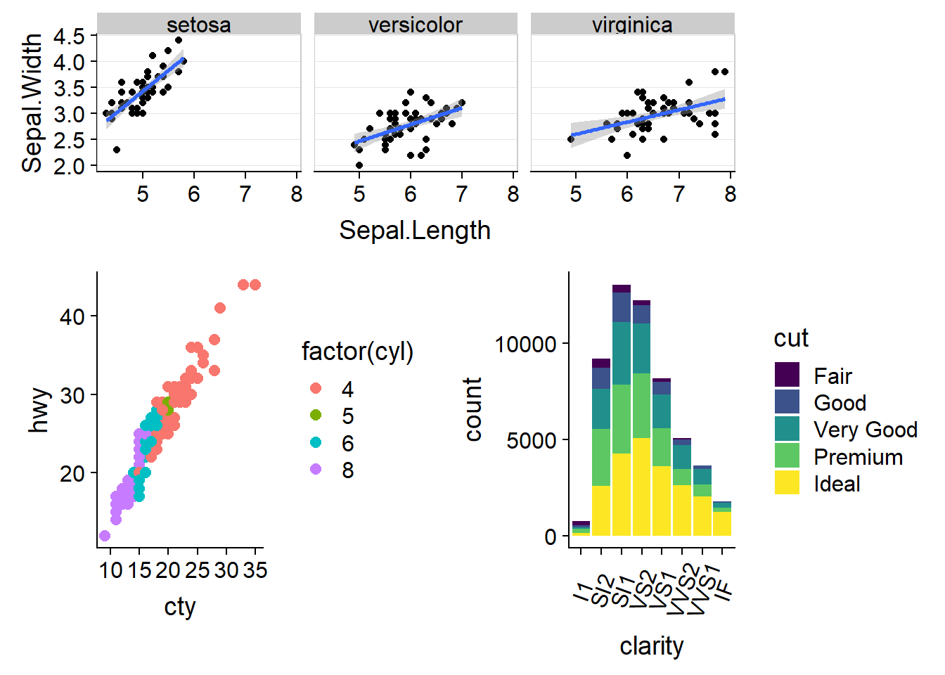
You can see that this aligns the edges of the plots rather than the legends, unlike in cowplot which has not aligned the histogram to the facetted plot.
Non ggplot objects
cowplot, unlike egg, can take non-ggplot objects - specifically gtable and recordedplot. The recordedplot class is from the recordPlot() function in the gridGraphics package and can represent many different plot types.
The recordPlot function takes a snapshot of the current plot, so first we plot out the plot we want then record it.
require(gridGraphics)
par(xpd = NA, # switch off clipping, necessary to always see axis labels
    bg = "transparent", # switch off background to avoid obscuring adjacent plots
    oma = c(2, 2, 0, 0), # move plot to the right and up
    mgp = c(2, 1, 0) # move axis labels closer to axis
  )
plot(sqrt) # plot the square root function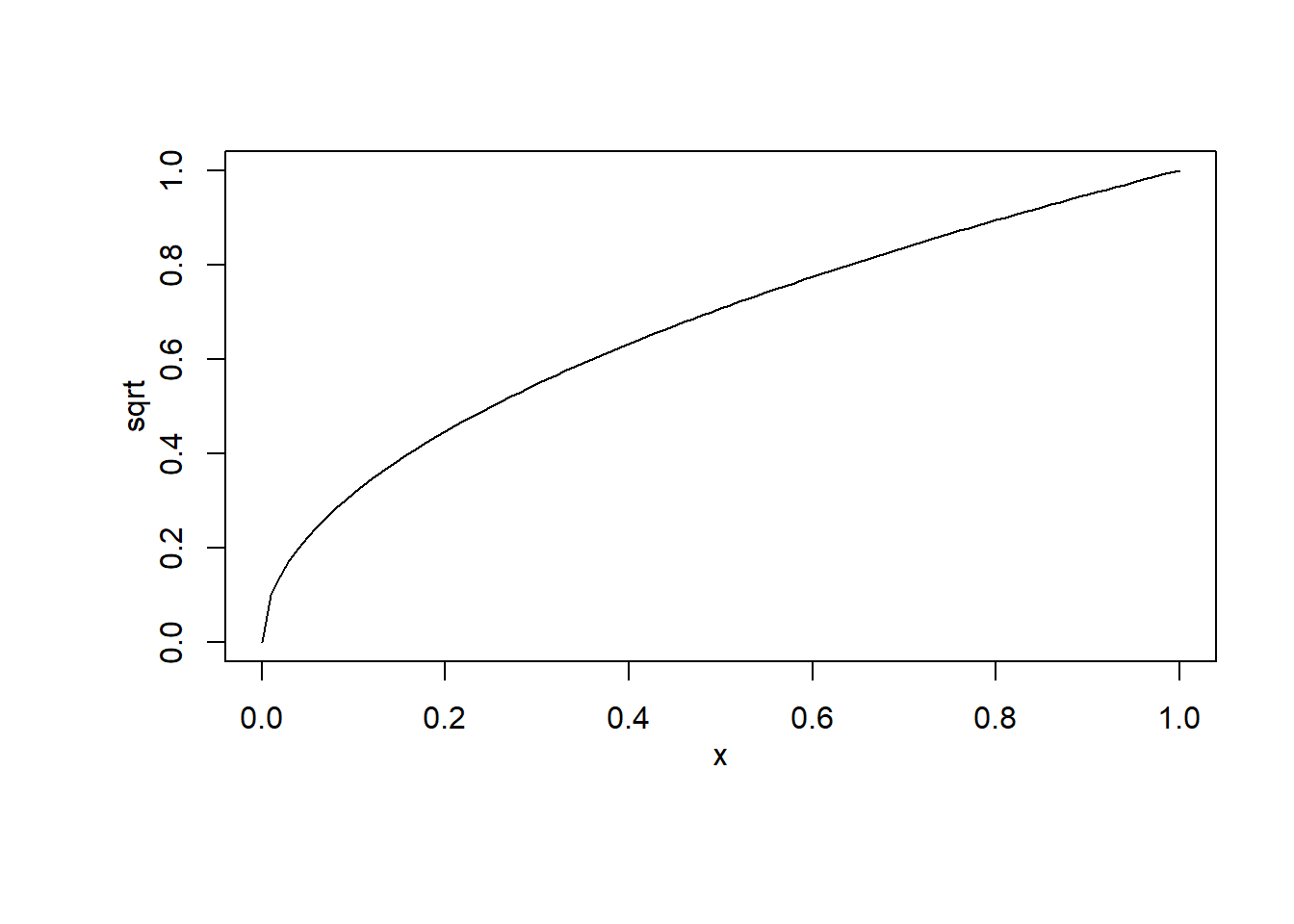
recordedplot <- recordPlot() The grid package has many built in functions which can directly draw things like circles or text, as we do here:
gtext <- grid::textGrob("Your ad here")We’re also going to use the ggdraw and draw_image functions within cowplot to create an image as a plot - this can also be used to add images on top of or behind plots, see the introduction vignette in cowplot for examples.
p3 <- ggdraw() + draw_image("https://jeroen.github.io/images/frink.png")Now we will combine these to create one big plot, using similar code to above. Note that we can’t align these types of plots.
left_col <- plot_grid(recordedplot, gtext, labels = c('A', 'B'), ncol = 1)
plot_grid(left_col, p3, labels = c('', 'C'), ncol = 2)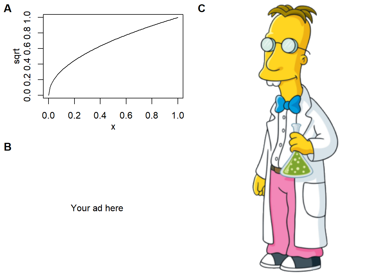
So that’s a few examples of how to create multi-panel plots using base R, cowplot and egg. A lot of this came from the cowplot vignettes, so I recommend taking a look at them for further information on arranging plots, sharing legends, changing the axis positions and plot annotations.