This tutorial is an introduction to simple linear regression in R, I’ve split it into two parts: this part is on modelling with numeric predictors.
First we’re going to load in all the packages we’ll be using in this analysis.
library(agridat)          # a package of agricultural datasets
library(summarytools)     # useful functions for summarising datasets
library(psych)            # more functions for examining datasets
library(dplyr)            # manipulating data
library(ggplot2)          # plotting
library(gridExtra)        # plotting in panels
library(car)              # extensions for regression
library(AICcmodavg)       # calculates AICc
As we’re plotting with ggplot I’m going to set the theme now for the whole tutorial to make it look nicer to me - see the plotting tutorial for more information on the plotting commands.
theme_set(theme_bw() + theme(panel.grid = element_blank()))Numerical predictors
We’re going to be using data from an experiment in 1952-3 looking at the impact of fertiliser application upon corn, clover and alfafa yields. A copy of the data is held in the agridat package, and the original analysis is linked to on the help page for the dataset. We’re going to read it in and take a quick look at it using the summarytools package:
Fert <- heady.fertilizer
# examining dataset using summarytools functions
print(dfSummary(Fert, style = 'grid', graph.magnif = 0.85), method = "render", omit.headings = TRUE)| No | Variable | Stats / Values | Freqs (% of Valid) | Graph | Valid | Missing | ||||||||||||||||||||||||||||||||||||||||||||||||||||||
|---|---|---|---|---|---|---|---|---|---|---|---|---|---|---|---|---|---|---|---|---|---|---|---|---|---|---|---|---|---|---|---|---|---|---|---|---|---|---|---|---|---|---|---|---|---|---|---|---|---|---|---|---|---|---|---|---|---|---|---|---|
| 1 | crop [factor] | 1. alfalfa 2. clover 3. corn 4. corn2 |
|
 |
648 (100%) | 0 (0%) | ||||||||||||||||||||||||||||||||||||||||||||||||||||||
| 2 | rep [integer] | Min : 1 Mean : 1.5 Max : 2 |
|
 |
648 (100%) | 0 (0%) | ||||||||||||||||||||||||||||||||||||||||||||||||||||||
| 3 | P [integer] | Mean (sd) : 160 (103.4) min < med < max: 0 < 160 < 320 IQR (CV) : 160 (0.6) |
|
 |
648 (100%) | 0 (0%) | ||||||||||||||||||||||||||||||||||||||||||||||||||||||
| 4 | K [integer] | Mean (sd) : 80 (108.4) min < med < max: 0 < 0 < 320 IQR (CV) : 160 (1.4) |
|
 |
648 (100%) | 0 (0%) | ||||||||||||||||||||||||||||||||||||||||||||||||||||||
| 5 | N [integer] | Mean (sd) : 80 (108.4) min < med < max: 0 < 0 < 320 IQR (CV) : 160 (1.4) |
|
|
648 (100%) | 0 (0%) | ||||||||||||||||||||||||||||||||||||||||||||||||||||||
| 6 | yield [numeric] | Mean (sd) : 31.5 (42.3) min < med < max: 1.1 < 4.2 < 144.9 IQR (CV) : 44.4 (1.3) | 326 distinct values |  |
456 (70.37%) | 192 (29.63%) |
Generated by summarytools 0.9.3 (R version 3.6.0)
2019-05-31
The different crops are all probably quite different in their responses, so we’re going to look at the summary statistics by group (again using the summarytools package, see the summary statistics tutorial for more methods).
# First save the results
by(data = Fert,
   INDICES = Fert$crop,
   FUN = descr, stats = c("mean", "sd", "min", "med", "max"),
   transpose = TRUE, style = "rmarkdown", omit.headings = TRUE)
## Fert$crop: alfalfa
## **Group:** crop = alfalfa
##
## | | Mean | Std.Dev | Min | Median | Max |
## |----------:|-------:|--------:|-----:|-------:|-------:|
## | **K** | 160.00 | 103.60 | 0.00 | 160.00 | 320.00 |
## | **N** | 0.00 | 0.00 | 0.00 | 0.00 | 0.00 |
## | **P** | 160.00 | 103.60 | 0.00 | 160.00 | 320.00 |
## | **rep** | 1.50 | 0.50 | 1.00 | 1.50 | 2.00 |
## | **yield** | 3.30 | 0.51 | 1.14 | 3.49 | 4.02 |
## --------------------------------------------------------
## Fert$crop: clover
## **Group:** crop = clover
##
## | | Mean | Std.Dev | Min | Median | Max |
## |----------:|-------:|--------:|-----:|-------:|-------:|
## | **K** | 160.00 | 103.60 | 0.00 | 160.00 | 320.00 |
## | **N** | 0.00 | 0.00 | 0.00 | 0.00 | 0.00 |
## | **P** | 160.00 | 103.60 | 0.00 | 160.00 | 320.00 |
## | **rep** | 1.50 | 0.50 | 1.00 | 1.50 | 2.00 |
## | **yield** | 3.45 | 0.40 | 2.29 | 3.54 | 4.31 |
## --------------------------------------------------------
## Fert$crop: corn
## **Group:** crop = corn
##
## | | Mean | Std.Dev | Min | Median | Max |
## |----------:|-------:|--------:|-----:|-------:|-------:|
## | **K** | 0.00 | 0.00 | 0.00 | 0.00 | 0.00 |
## | **N** | 160.00 | 103.60 | 0.00 | 160.00 | 320.00 |
## | **P** | 160.00 | 103.60 | 0.00 | 160.00 | 320.00 |
## | **rep** | 1.50 | 0.50 | 1.00 | 1.50 | 2.00 |
## | **yield** | 86.07 | 46.35 | 4.20 | 106.35 | 144.90 |
## --------------------------------------------------------
## Fert$crop: corn2
## **Group:** crop = corn2
##
## | | Mean | Std.Dev | Min | Median | Max |
## |----------:|-------:|--------:|-----:|-------:|-------:|
## | **K** | 0.00 | 0.00 | 0.00 | 0.00 | 0.00 |
## | **N** | 160.00 | 103.60 | 0.00 | 160.00 | 320.00 |
## | **P** | 160.00 | 103.60 | 0.00 | 160.00 | 320.00 |
## | **rep** | 1.50 | 0.50 | 1.00 | 1.50 | 2.00 |
## | **yield** | 33.03 | 21.29 | 3.70 | 28.45 | 76.70 |We’re going to treat the fertiliser treatments as numeric as there are sufficient different treatments to fit linear regression, and for ease of interpretation.
Let’s take the response of clover to fertilisation, first we’ll filter out the rows that correspond to clover and use droplevels to get rid of the empty levels within the crop variable. We’ll use pairs.panels from the psych package to take a quick look at the relationships between the variables.
clover <- filter(Fert, crop == "clover")
clover <- droplevels(clover)
pairs.panels(clover[,c(2,3,4,6)])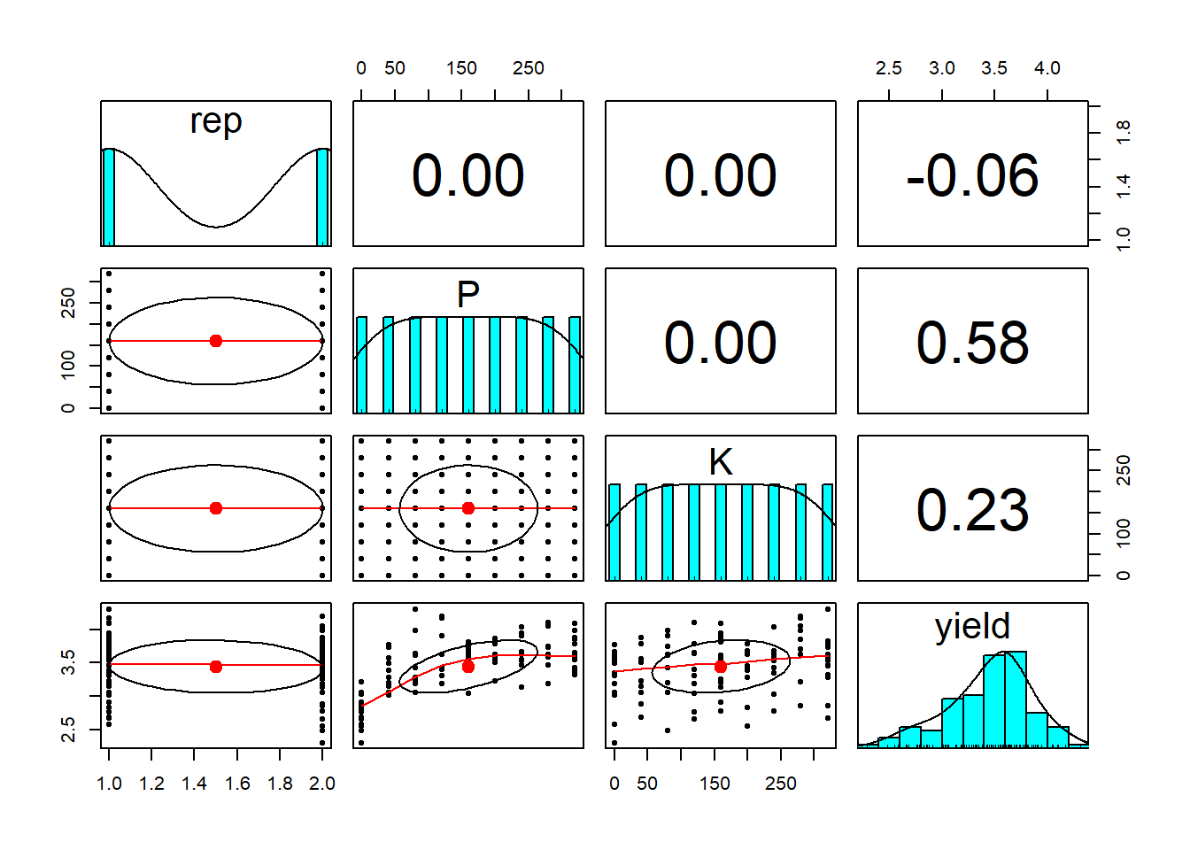
We can see there is no correlation between the treatments, as expected as this experiment was designed that way. There was no nitrogen added to the clover crops as clover is nitrogen fixing so we’re only looking at the impact of P and K fertiliser addition. We’ll plot more detailed plots of the yield against the P and K fertiliser use using ggplot.
(Pplot <- ggplot(clover, aes(x=P, y=yield)) +
    geom_point() +
    labs(x = "Phosphorus (pounds/acre)", y = "Yield (tons/acre)") +
    geom_smooth(method="lm"))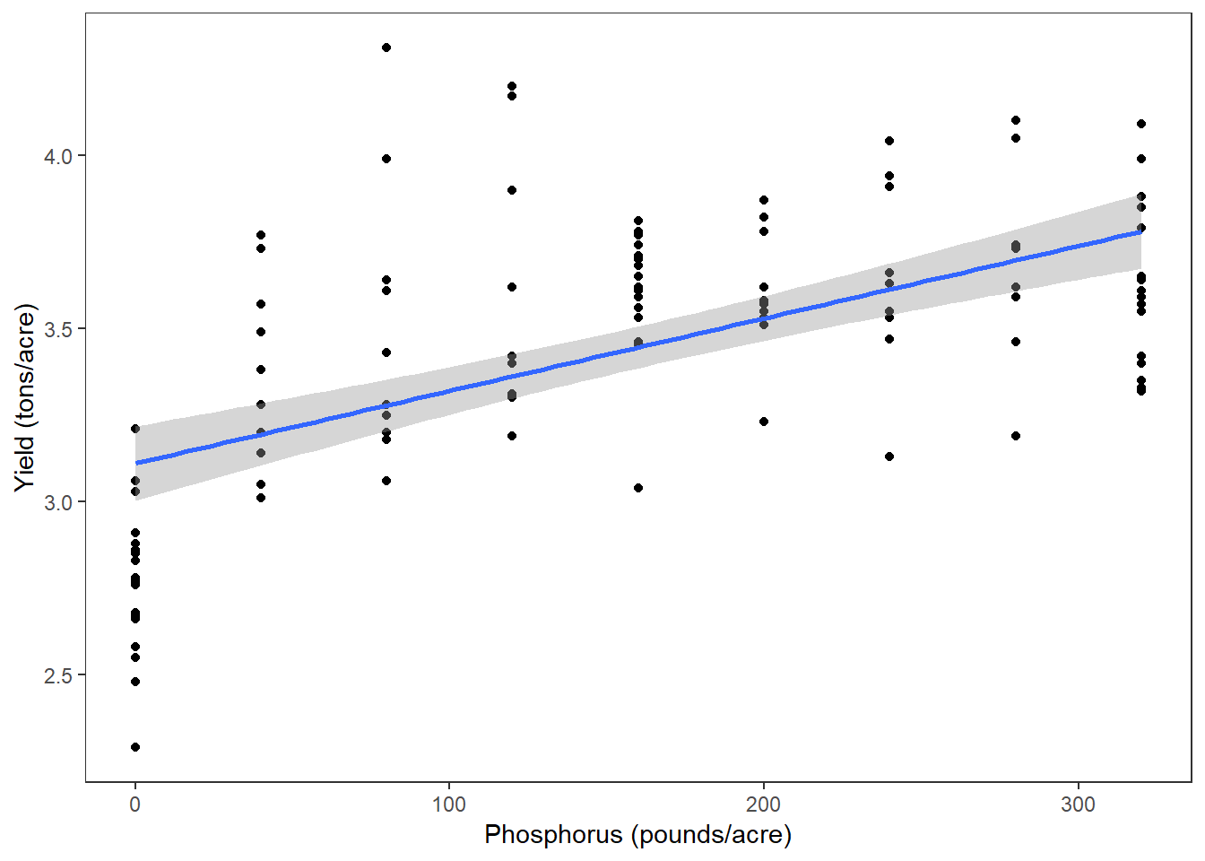
(Kplot <- ggplot(clover, aes(x=K, y=yield)) +
    geom_point() +
    labs(x = "Potassium (pounds/acre)", y = "Yield (tons/acre)") +
    geom_smooth(method="lm"))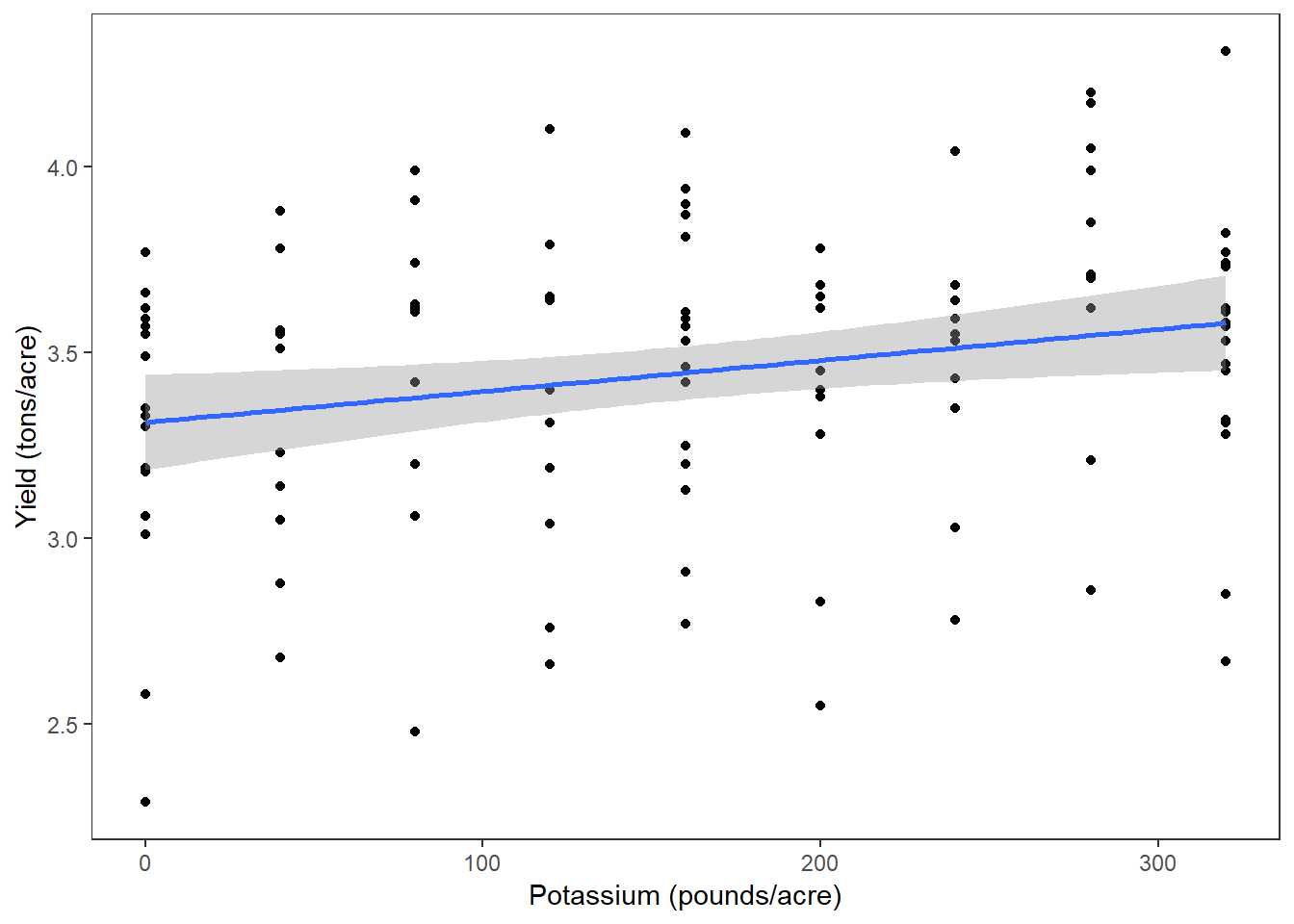
grid.arrange(Pplot, Kplot, nrow=1)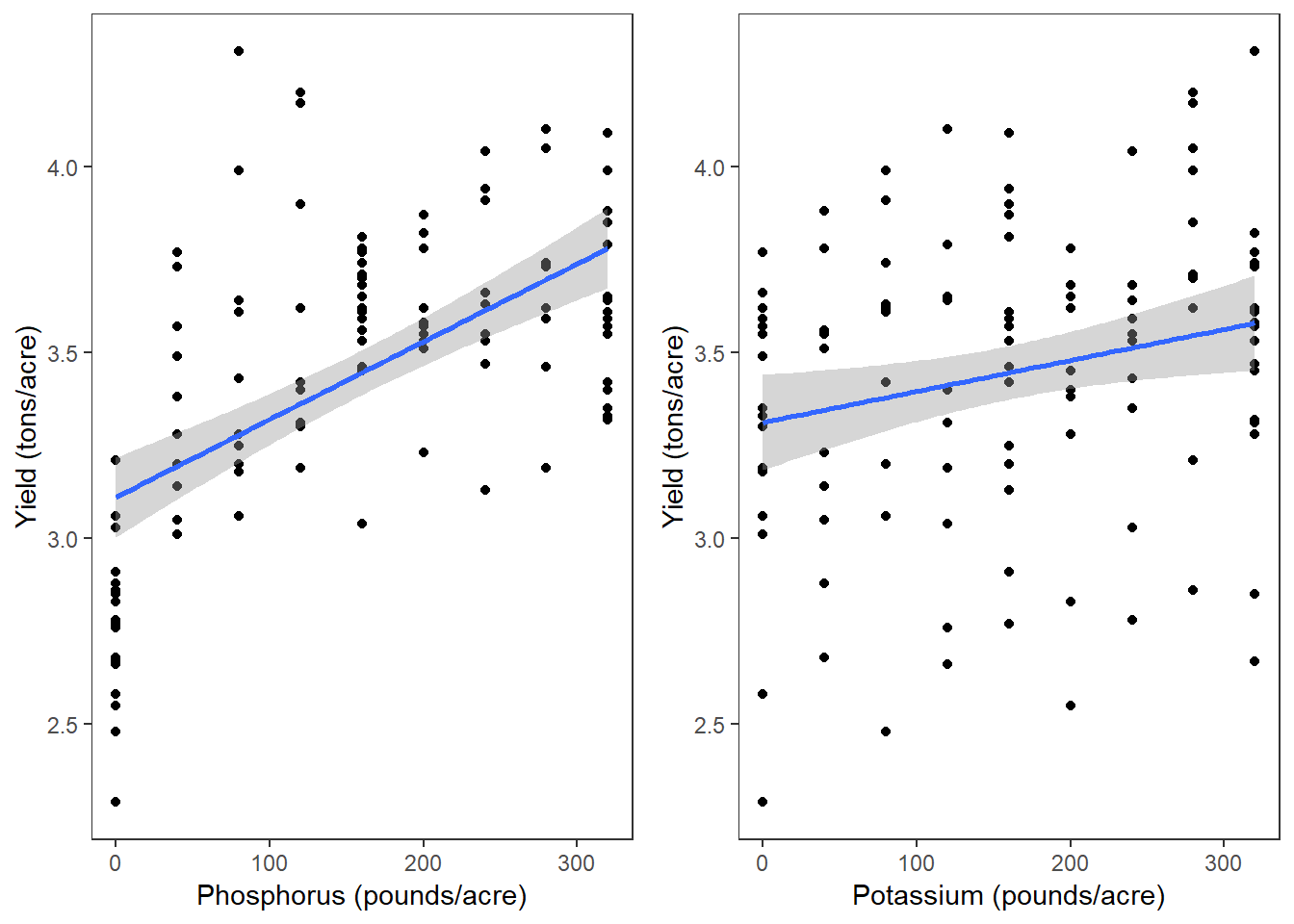
Now we want to fit our linear model and see if yield increases with fertiliser use. First we’re going to fit each fertiliser treatment separately, for demonstratory purposes.
cloverp.lm <- lm(yield ~ P, clover)
summary(cloverp.lm)
##
## Call:
## lm(formula = yield ~ P, data = clover)
##
## Residuals:
## Min 1Q Median 3Q Max
## -0.82080 -0.20802 0.00309 0.22818 1.03179
##
## Coefficients:
## Estimate Std. Error t value Pr(>|t|)
## (Intercept) 3.110801 0.053920 57.693 < 2e-16 ***
## P 0.002093 0.000278 7.527 1.41e-11 ***
## ---
## Signif. codes: 0 '***' 0.001 '**' 0.01 '*' 0.05 '.' 0.1 ' ' 1
##
## Residual standard error: 0.3254 on 112 degrees of freedom
## (48 observations deleted due to missingness)
## Multiple R-squared: 0.3359, Adjusted R-squared: 0.33
## F-statistic: 56.65 on 1 and 112 DF, p-value: 1.415e-11We can see from the bottom lines of the output that P fertiliser has a significant impact upon clover yield at p = 1.415e-11, the F statistic is usually reported as well. Here we’d say that F1,112=56.65. The R2 value is 0.336, which seems promising for crop research!
Whenever you do a linear model make sure to check the assumptions! You can plot the model which will return four graphs: the qqplot, the residuals against fitted values, the standardised residuals against fitted values, and the leverage plot. We want the points in the qqplot to lie near the qqline, if they don’t then the assumption of normality of residuals is violated. If there residuals appear to change consistently with the fitted values then that could mean the assumption of homoscedasticity, or homogeneity of variance, is violated which can be a big problem in model fitting. Here I’ve used par to set graphical parameters so you get two four plots in a 2x2 matrix then reverted to the previous setting.
par(mfrow=c(2,2));plot(cloverp.lm);par(mfrow=c(1,1))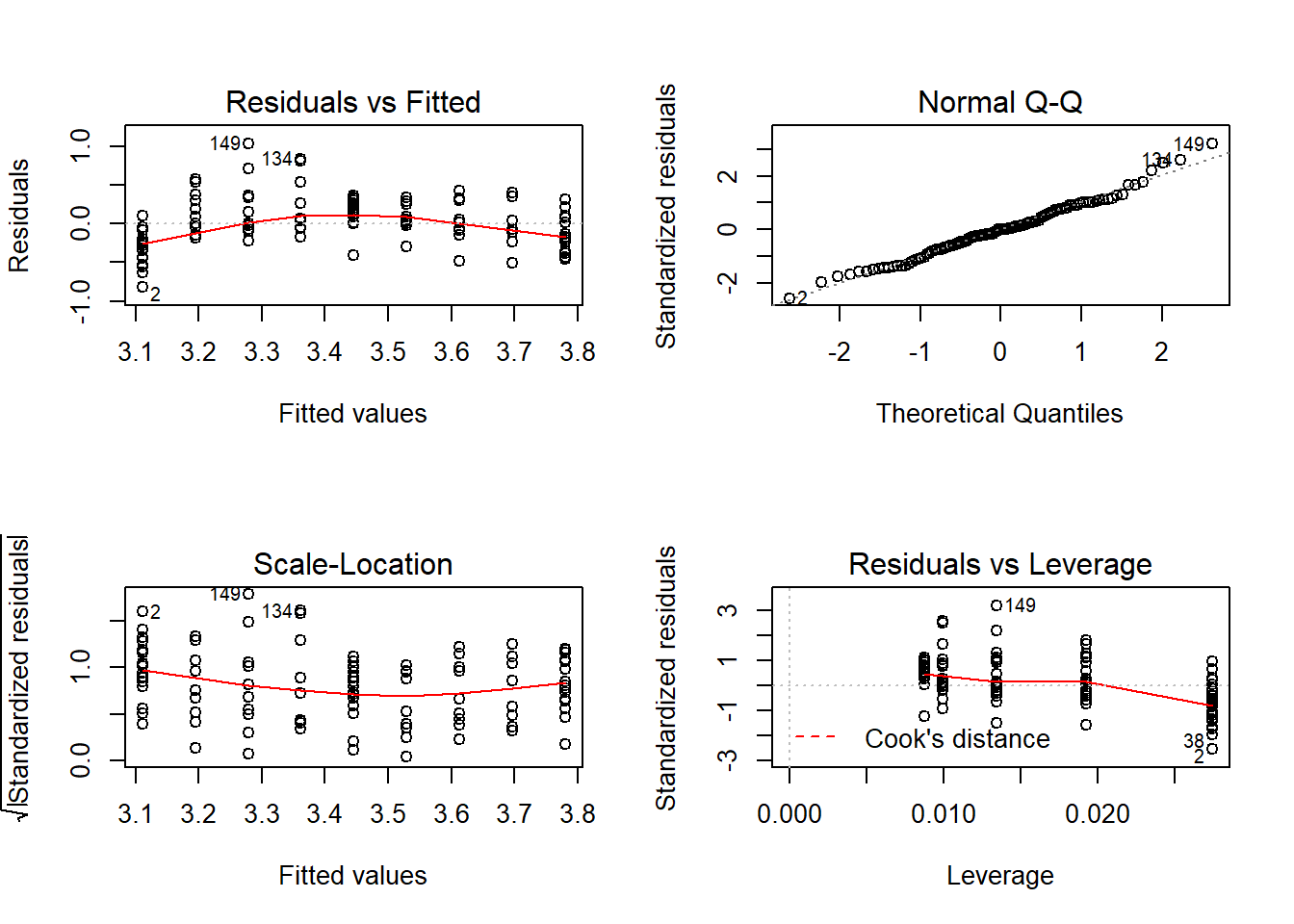
It can be difficult to interpret diagnostic plots sometimes, and I’ve found the qqp function within the car package very useful as it gives confidence intervals around the qqline so you can see more clearly which points are a problem.
qqp(cloverp.lm)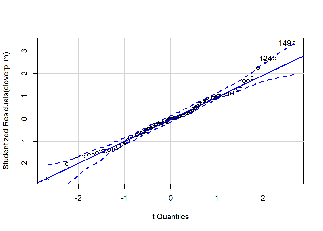
## [1] 134 149Now we’re going to repeat the above for K fertiliser addition! First, model fitting:
cloverk.lm <- lm(yield ~ K, clover)
summary(cloverk.lm)
##
## Call:
## lm(formula = yield ~ K, data = clover)
##
## Residuals:
## Min 1Q Median 3Q Max
## -1.02188 -0.20374 0.03939 0.23812 0.73065
##
## Coefficients:
## Estimate Std. Error t value Pr(>|t|)
## (Intercept) 3.3118757 0.0643688 51.452 <2e-16 ***
## K 0.0008359 0.0003319 2.518 0.0132 *
## ---
## Signif. codes: 0 '***' 0.001 '**' 0.01 '*' 0.05 '.' 0.1 ' ' 1
##
## Residual standard error: 0.3884 on 112 degrees of freedom
## (48 observations deleted due to missingness)
## Multiple R-squared: 0.0536, Adjusted R-squared: 0.04515
## F-statistic: 6.343 on 1 and 112 DF, p-value: 0.0132There doesn’t appear to be much of an impact of K fertiliser on yield, p is significant but the R2 is very low.
Now, model checking:
par(mfrow=c(2,2));plot(cloverk.lm);par(mfrow=c(1,1))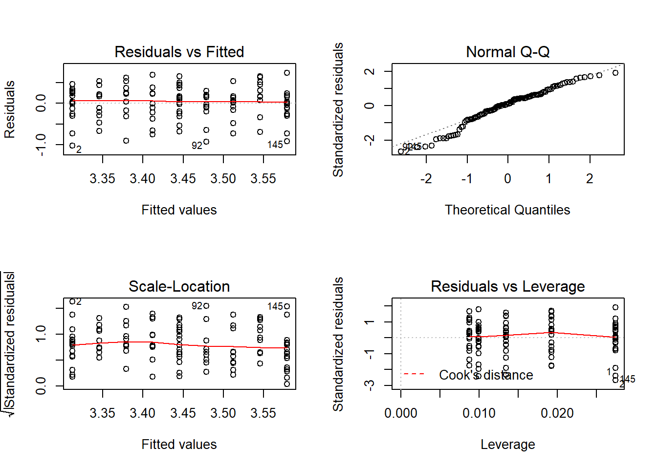
qqp(cloverk.lm)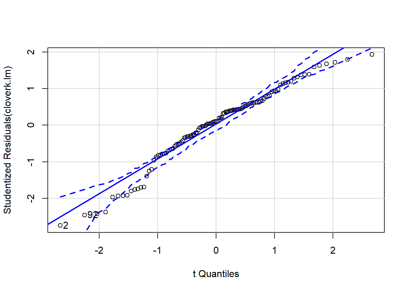
## [1] 2 92Now often we don’t expect a linear response, and we can fit polynomial models using lm. I’ll show you how to fit a quadratic function, there’s code in the heady.fertiliser help file that shows how they fit models with square root terms.
cloverp.lm2 <- lm(yield ~ I(P^2) + P, clover)
summary(cloverp.lm2)
##
## Call:
## lm(formula = yield ~ I(P^2) + P, data = clover)
##
## Residuals:
## Min 1Q Median 3Q Max
## -0.60457 -0.17493 -0.03652 0.12533 0.93882
##
## Coefficients:
## Estimate Std. Error t value Pr(>|t|)
## (Intercept) 2.886e+00 5.722e-02 50.430 < 2e-16 ***
## I(P^2) -1.656e-05 2.513e-06 -6.589 1.54e-09 ***
## P 7.392e-03 8.384e-04 8.817 1.87e-14 ***
## ---
## Signif. codes: 0 '***' 0.001 '**' 0.01 '*' 0.05 '.' 0.1 ' ' 1
##
## Residual standard error: 0.2771 on 111 degrees of freedom
## (48 observations deleted due to missingness)
## Multiple R-squared: 0.5226, Adjusted R-squared: 0.514
## F-statistic: 60.76 on 2 and 111 DF, p-value: < 2.2e-16par(mfrow=c(2,2));plot(cloverp.lm2);par(mfrow=c(1,1))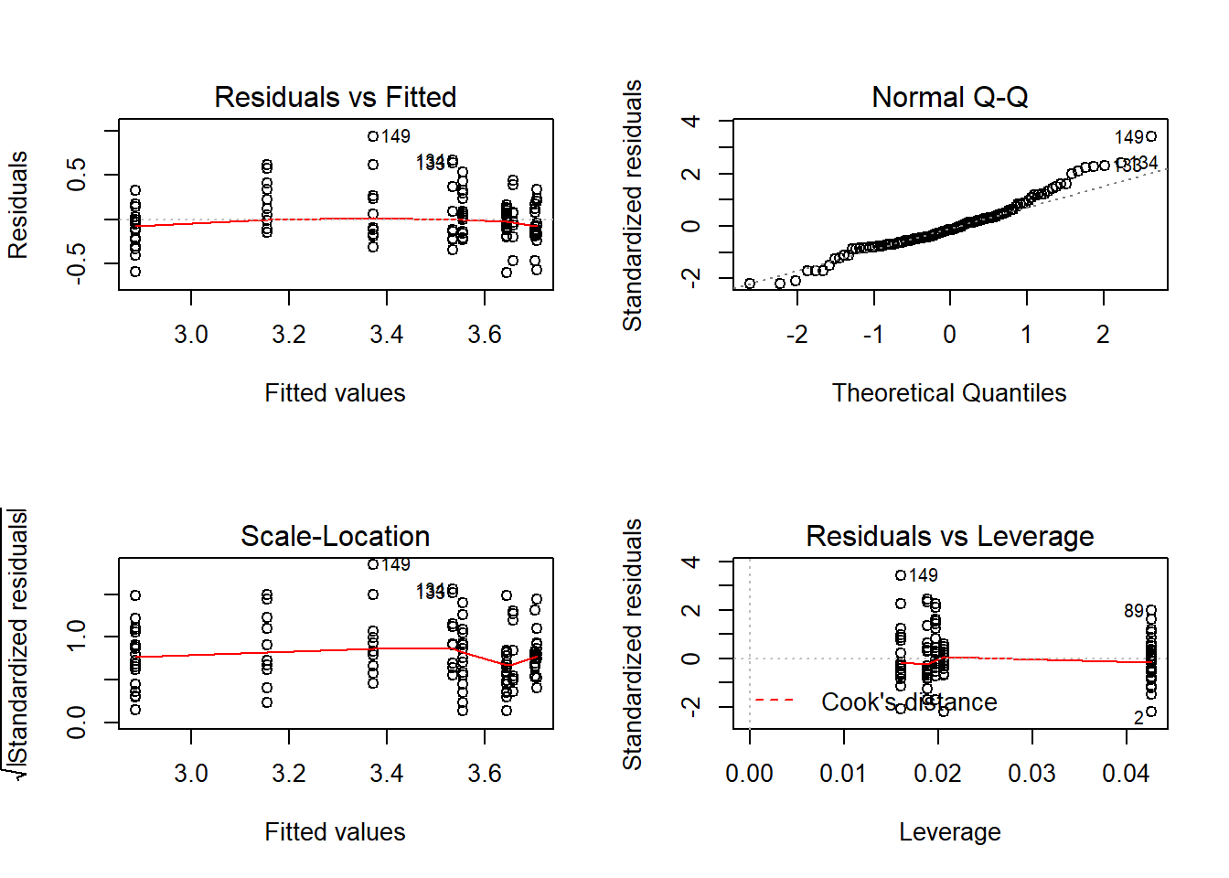
qqp(cloverp.lm2)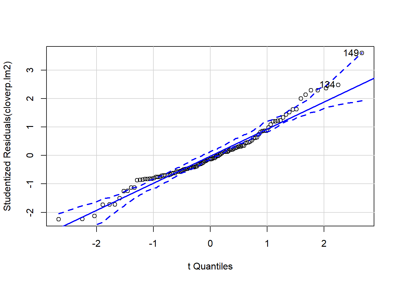
## [1] 134 149Two predictors
Now this experiment involved adding the two fertilisers together and separately so we should be taking both treatments into account and fitting models with two predictors. First we can use an asterisk to estimate if there’s some kind of interaction effect between the predictors.
cloverpk.lm <- lm(yield ~ K*P, clover)
summary(cloverpk.lm)
##
## Call:
## lm(formula = yield ~ K * P, data = clover)
##
## Residuals:
## Min 1Q Median 3Q Max
## -0.65579 -0.20341 0.00423 0.18278 0.86017
##
## Coefficients:
## Estimate Std. Error t value Pr(>|t|)
## (Intercept) 2.902e+00 9.213e-02 31.501 < 2e-16 ***
## K 1.324e-03 4.811e-04 2.752 0.00693 **
## P 2.605e-03 4.811e-04 5.414 3.65e-07 ***
## K:P -3.295e-06 2.497e-06 -1.319 0.18985
## ---
## Signif. codes: 0 '***' 0.001 '**' 0.01 '*' 0.05 '.' 0.1 ' ' 1
##
## Residual standard error: 0.3136 on 110 degrees of freedom
## (48 observations deleted due to missingness)
## Multiple R-squared: 0.3942, Adjusted R-squared: 0.3777
## F-statistic: 23.86 on 3 and 110 DF, p-value: 5.716e-12par(mfrow=c(2,2));plot(cloverpk.lm);par(mfrow=c(1,1))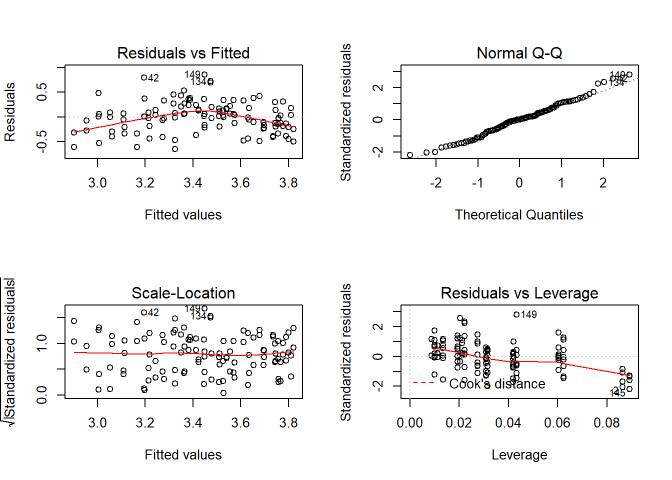
qqp(cloverpk.lm)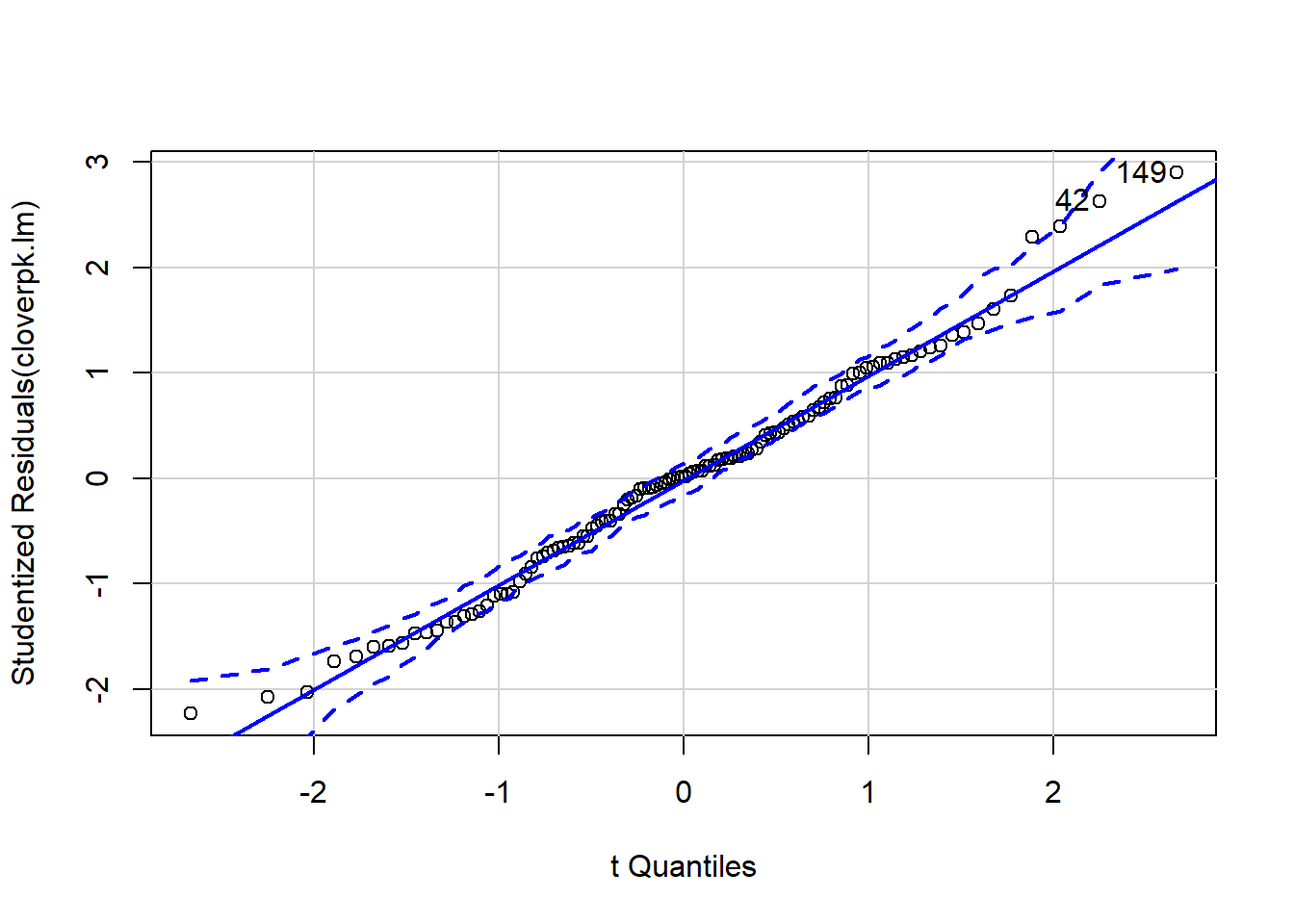
## [1] 42 149Here we can see that this model is significant at p < 0.0001, and it has the highest R2 yet! However notice that if you look at the coefficients the interaction effect (K:P) is low, and p = 0.19. We can try fitting the model without this interaction and see what happens:
cloverpk.lm2 <- lm(yield ~ K + P, clover)
summary(cloverpk.lm2)
##
## Call:
## lm(formula = yield ~ K + P, data = clover)
##
## Residuals:
## Min 1Q Median 3Q Max
## -0.69566 -0.20316 0.00249 0.19212 0.90308
##
## Coefficients:
## Estimate Std. Error t value Pr(>|t|)
## (Intercept) 2.9856599 0.0670865 44.505 < 2e-16 ***
## K 0.0007970 0.0002689 2.964 0.00371 **
## P 0.0020777 0.0002689 7.727 5.3e-12 ***
## ---
## Signif. codes: 0 '***' 0.001 '**' 0.01 '*' 0.05 '.' 0.1 ' ' 1
##
## Residual standard error: 0.3146 on 111 degrees of freedom
## (48 observations deleted due to missingness)
## Multiple R-squared: 0.3846, Adjusted R-squared: 0.3735
## F-statistic: 34.69 on 2 and 111 DF, p-value: 1.983e-12par(mfrow=c(2,2));plot(cloverpk.lm2);par(mfrow=c(1,1))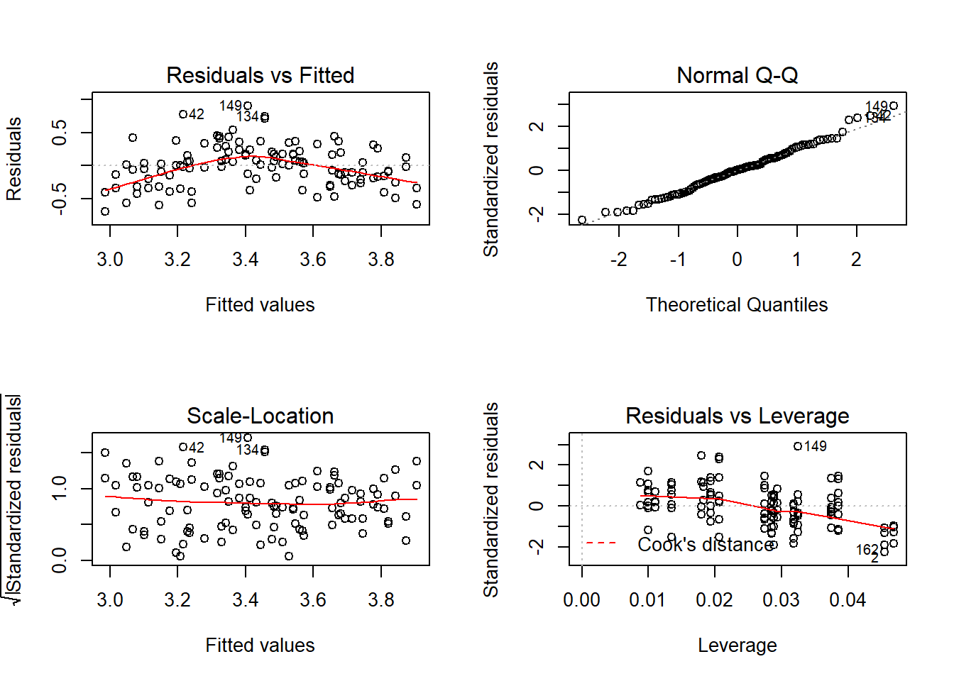
qqp(cloverpk.lm2)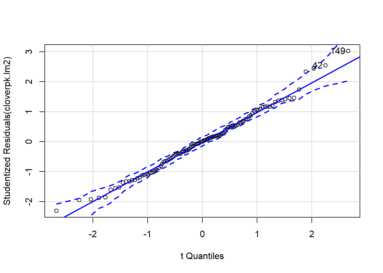
## [1] 42 149This model looks fairly similar in R2 to the previous, however it is better practice to compare models using an information criterion. Information criterions look at how much variation is explained by the model and then penalise for model complexity. Therefore if two models explain the same amount of variation then the simpler model will be preferred. One of the most common ICs is AIC (Aikake’s An Information Criterion). This is present in base R, but we’re going to use a version that works better with small sample sizes: AICc. We’ll use the AICcmodavg package to do this.
AICc(cloverpk.lm) ## [1] 65.58202AICc(cloverpk.lm2) ## [1] 65.18282AICc(cloverp.lm)## [1] 71.71905AICc(cloverk.lm)## [1] 112.1038A commonly used rule of thumb is that if the AIC(c)’s are within 2 points of each other the models are essentially equivalent. We have a difference of 0.4 between the two models with both P and K as predictors so these are essentially equivalent. The model with P only is noticeably worse, and K doesn’t do well at all.
One more diagnostic check for models with multiple predictors!
If the predictors are highly correlated then the model struggles to estimate impact and estimated error of coefficients will be high. VIF estimates the influence of multicollinearity on estimated variance of predictors.
vif(cloverpk.lm2)## K P
## 1.000349 1.000349For more on vif see http://www.statisticshowto.com/variance-inflation-factor/ Rough rules: VIF=1 not correlated; 1<VIF<5 moderately correlated; VIF>5 highly correlated. vif here is low, as we’d expect with a correlation coefficient of 0 between P and K